Something Fishy This Way Comes: Fish Segmentation in Mathematica

EEE 533

Overview

This project focused on recovering the segmentation mask of a fish from a photograph taken on a green measuring board. The submitted algorithm was evaluated on three statistics derived from that segmentation: area, centroid, and the horizontal length of the fish in pixels. The core challenge was to make that pipeline robust to the actual conditions in the dataset rather than only to a single clean example. The fish sits on a structured green measuring board, but reflections, shadows, transparent fins, and background-connected artifacts make the segmentation problem less trivial than it first appears.

What made the project interesting was that the task naturally combined two levels of reasoning. At the segmentation stage, the goal was to isolate the fish reliably using the color and geometric structure of the scene. At the measurement stage, the result had to be stable enough that the same mask could support downstream quantities like centroid and size-related statistics without collapsing under small boundary errors. That made the project a good exercise in building an interpretable classical vision pipeline rather than a one-off thresholding trick.

Problem framing

The image setup provides a useful prior: most of the background is the green measuring board, while the fish occupies a single dominant interior region. But the data is structured rather than clean. Parts of the board become bright under reflection, fins can appear faint or semi-transparent, and some unwanted regions remain connected to the image border even after coarse masking. A good solution therefore has to use the board prior without assuming that color alone will separate foreground from background perfectly.

The project output was not just the segmented fish itself. The notebook also measures area, centroid, and the fish’s horizontal length from the recovered mask. That requirement changes the problem slightly. The objective is not only to produce a visually plausible segmentation, but to recover a mask whose shape is stable enough for geometric measurement. In practice, that means the pipeline has to preserve the main fish body, reject background-connected clutter, and avoid introducing holes or fragmentation that would distort the final statistics.

Final pipeline

The final version of the pipeline treats the task as a sequence of increasingly stricter filters. I tried to exploit the fact that the back board is green as much as possible, but that prior alone was not enough. The pipeline first isolates the parts of the image that behave differently from the green measuring board, then combines those cues into a candidate fish region, and finally removes any leftover structures that are too small or still connected to the image boundary. What makes the approach effective is not any single threshold by itself, but the way the stages reinforce one another.

The remastered notebook makes that process visible on one representative sample, so the chapter below shows the full flow from raw image to final mask.

1. Input and reference mask

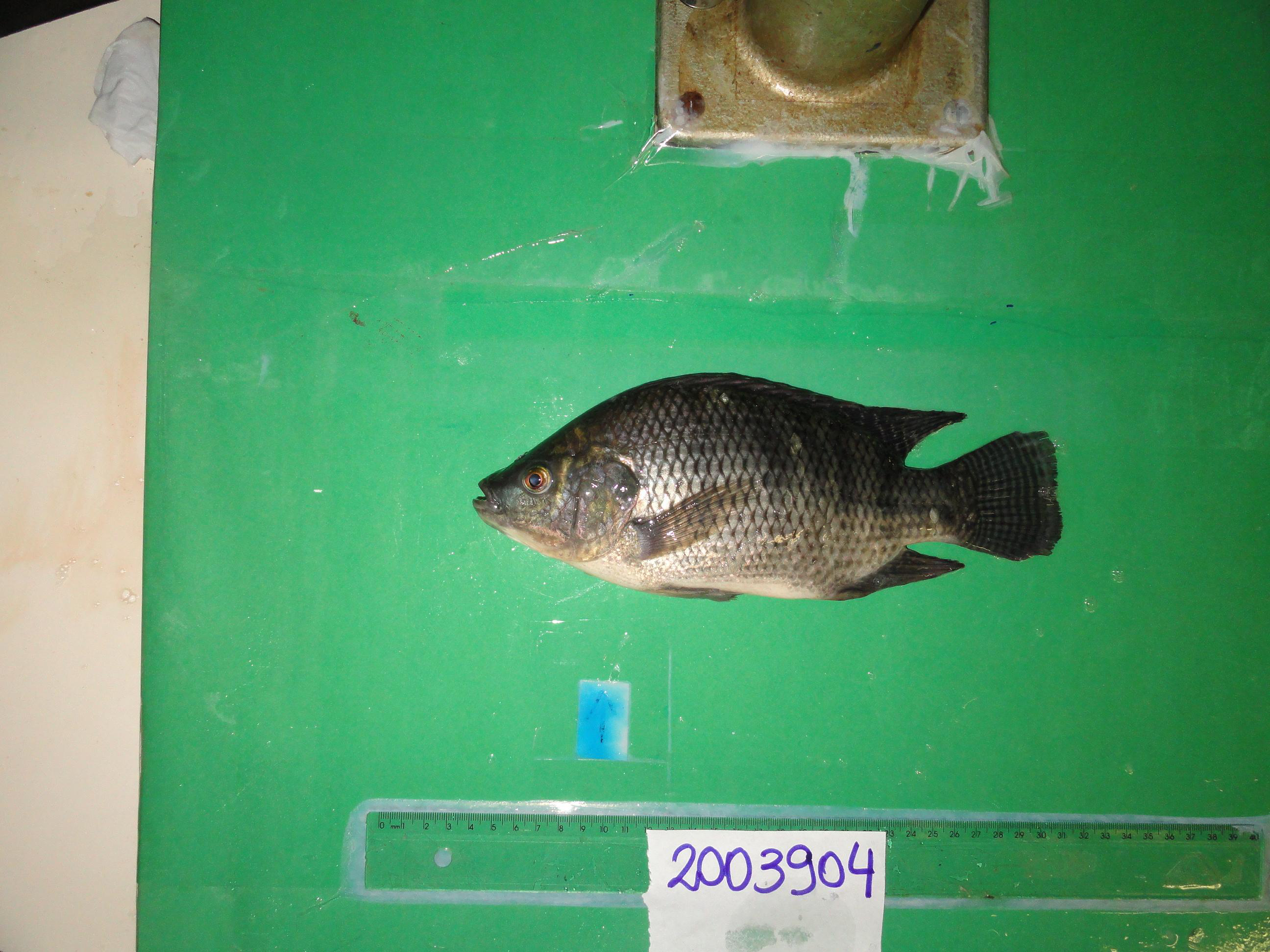
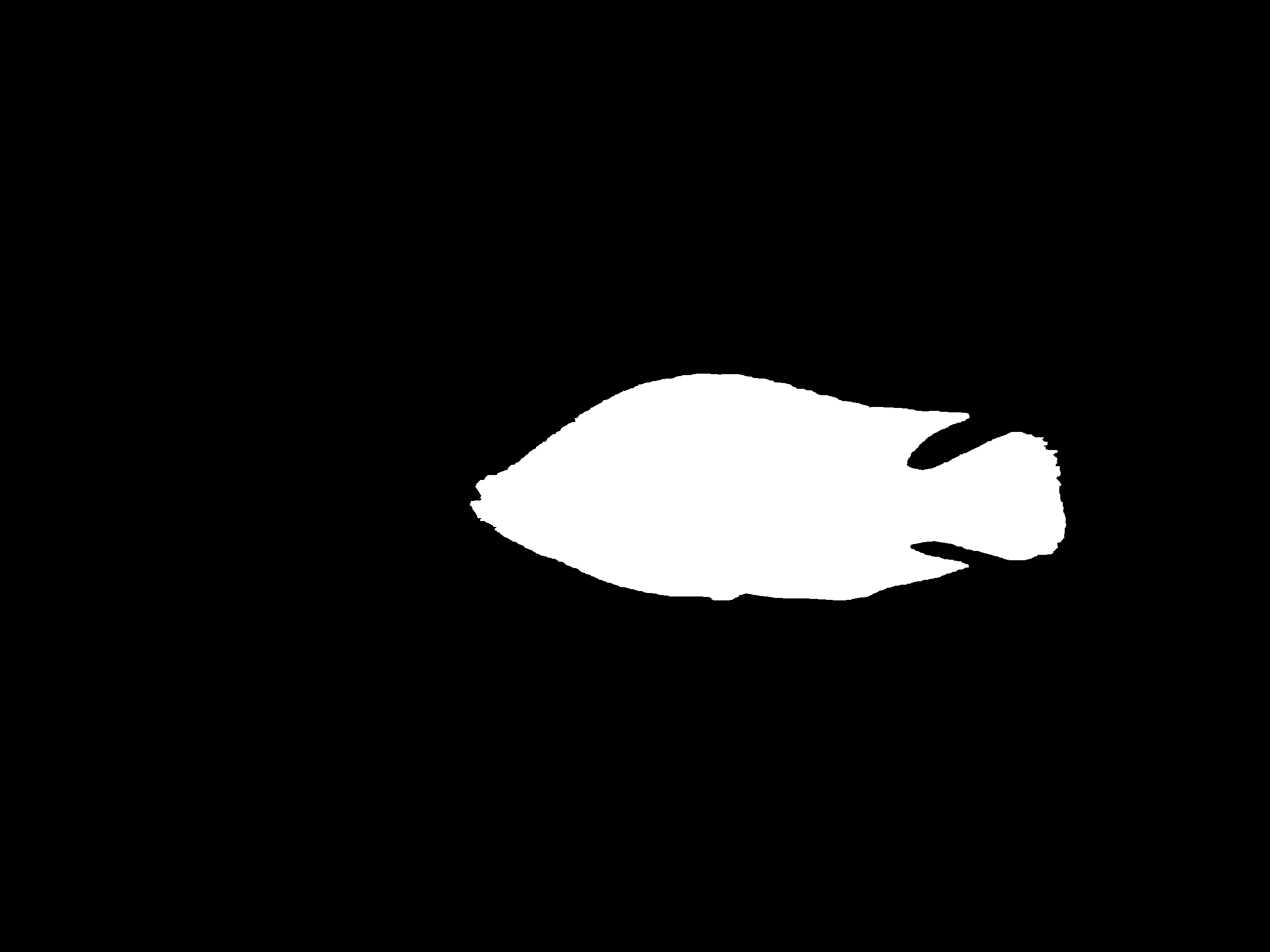
The pipeline starts from a fish image on a mostly green board and compares its output against a reference mask for that same fish. The goal is to recover the same silhouette automatically, even though the raw image includes glare, shadows, and semi-transparent fin regions.

2. HSB decomposition

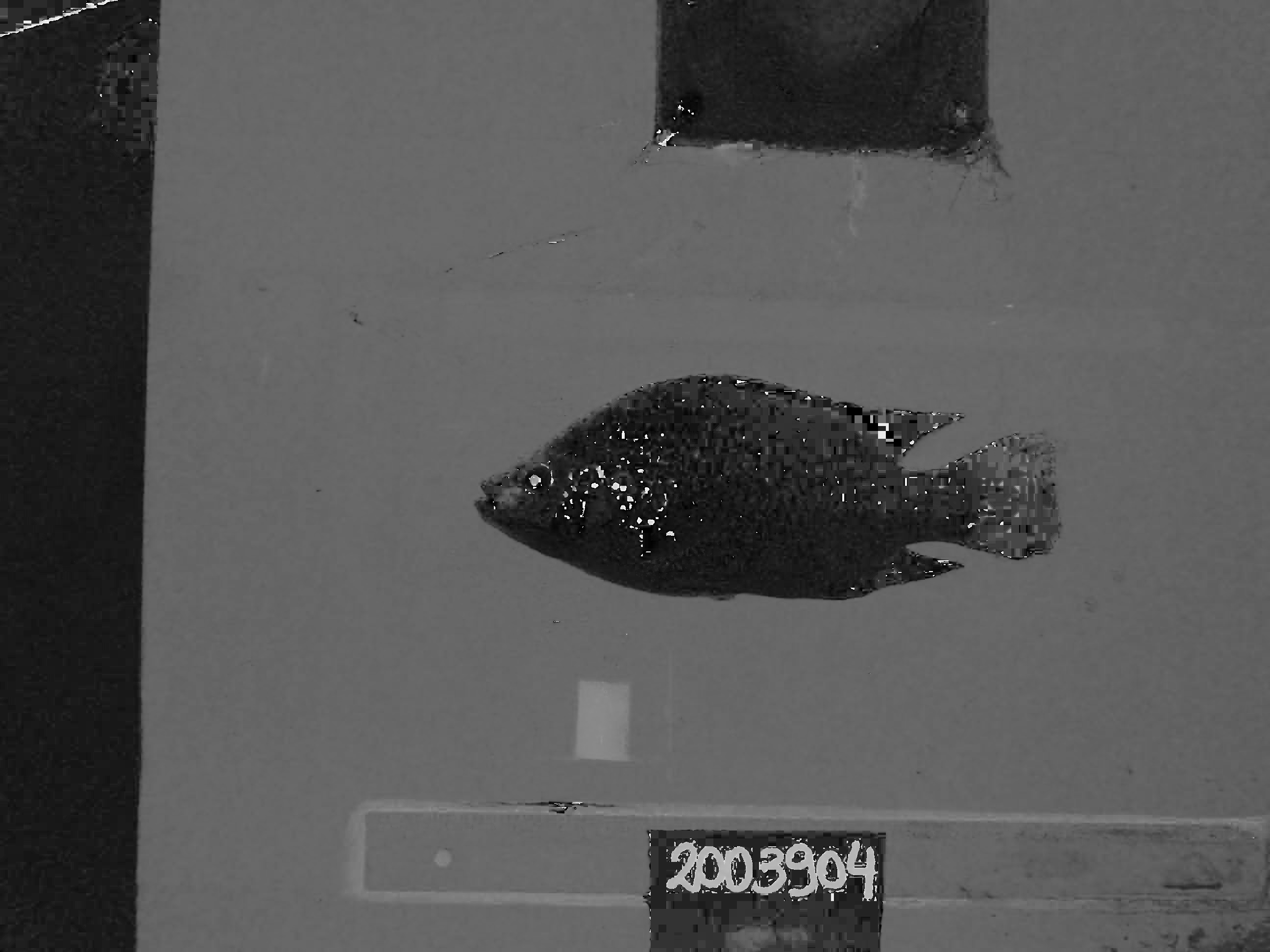
The first step is to view the image through hue, saturation, and brightness separately. This makes the structure of the problem much clearer. The board is most obvious in hue, reflective clutter shows up differently in brightness, and saturation helps preserve fish texture that would be ambiguous in a single grayscale view.

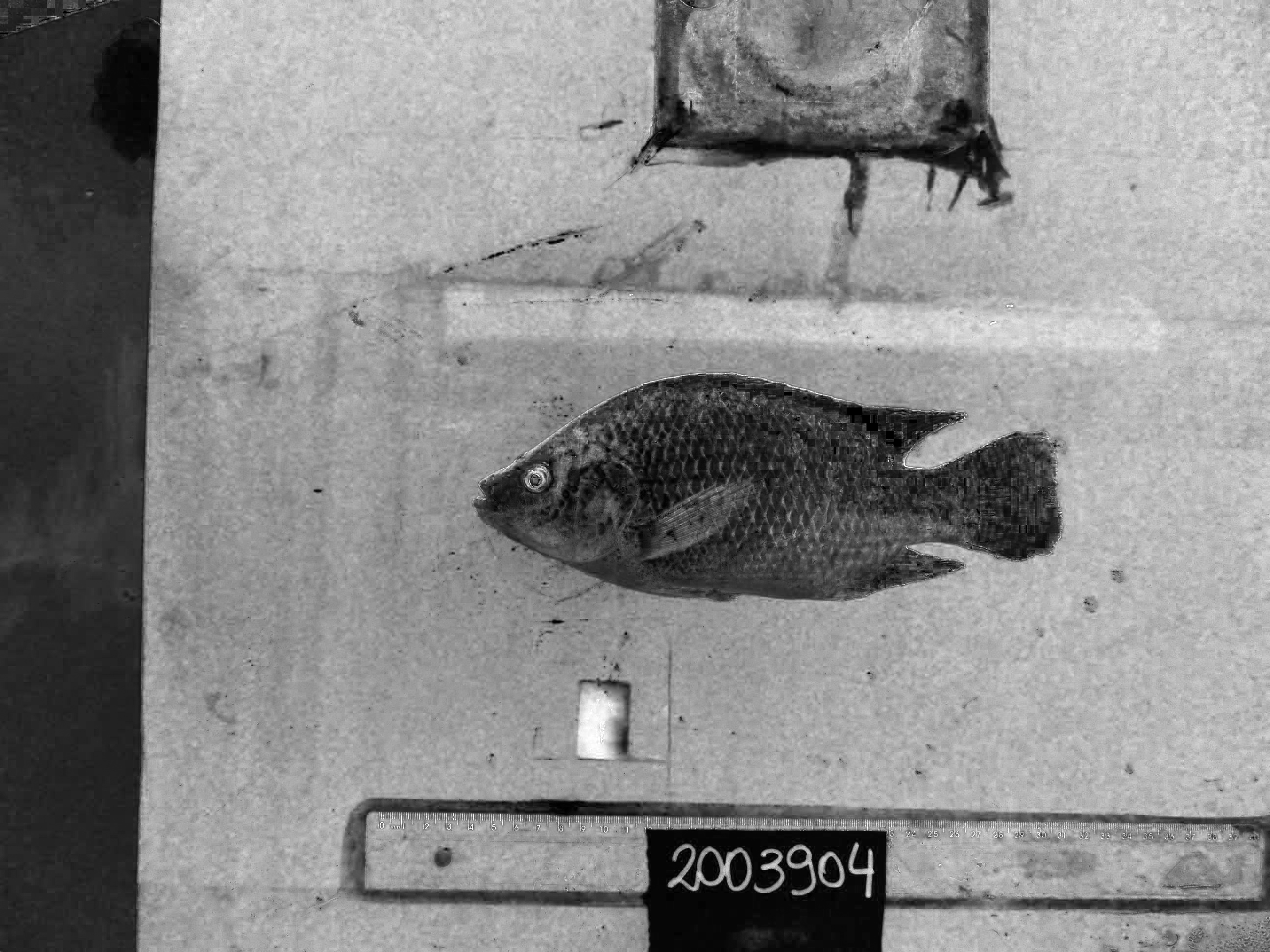
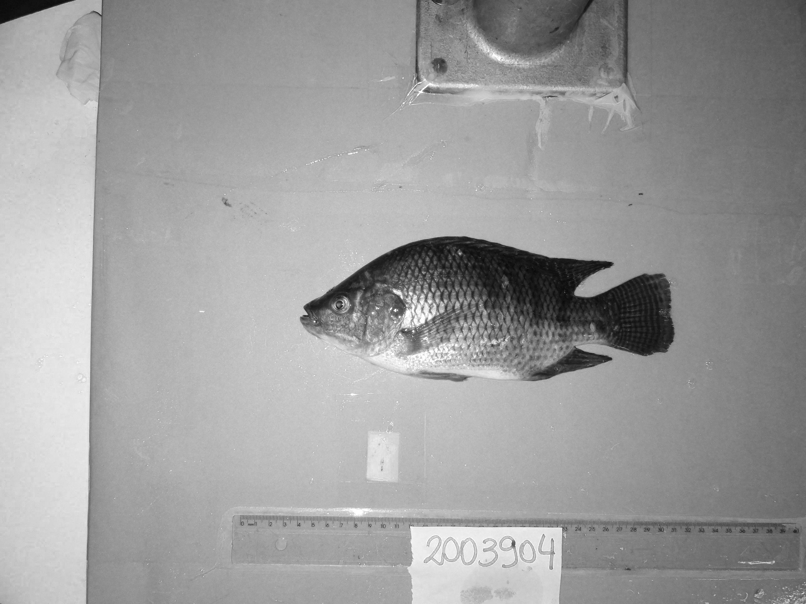
3. Per-channel thresholding

Once the three channels are separated, each one is filtered with a range chosen for its role in the task. Hue keeps the board prior explicit, saturation protects the fish body from disappearing into the background, and brightness suppresses high-glare regions that would otherwise contaminate the mask.

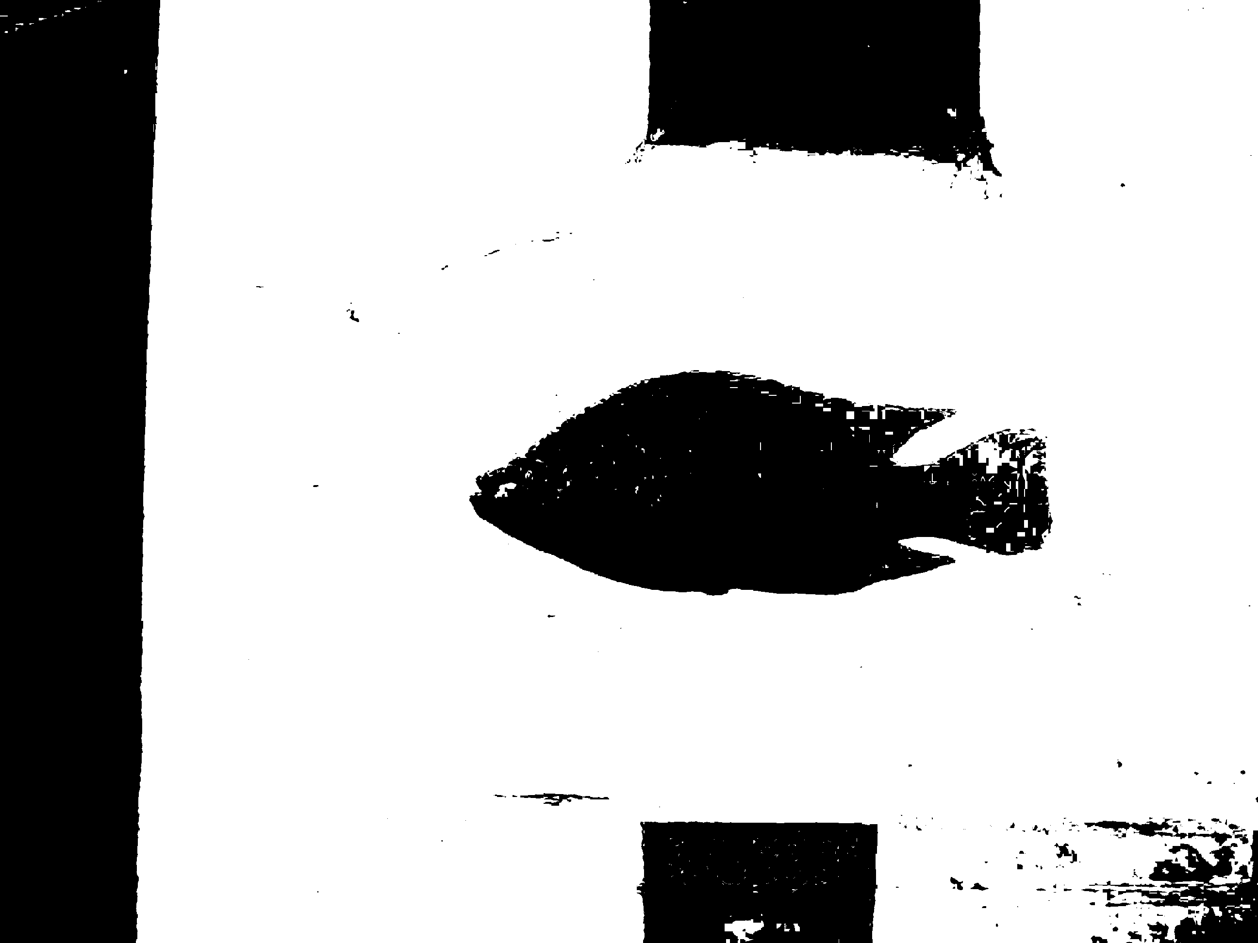
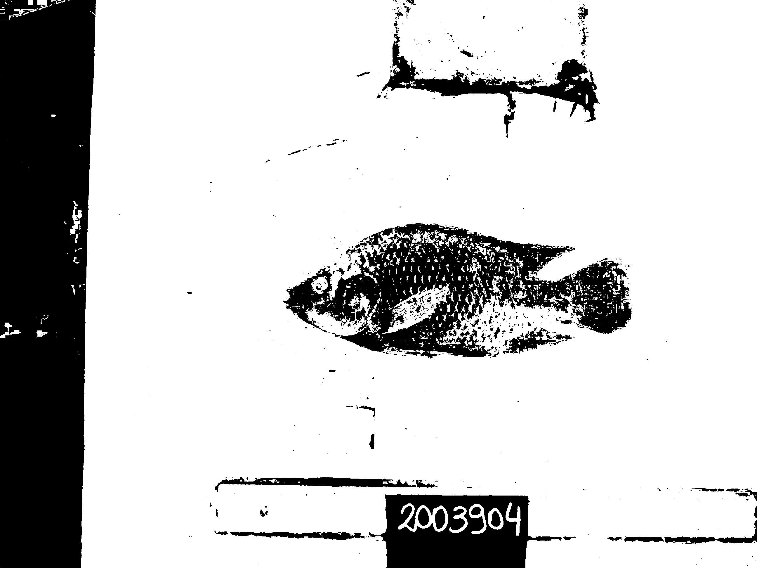
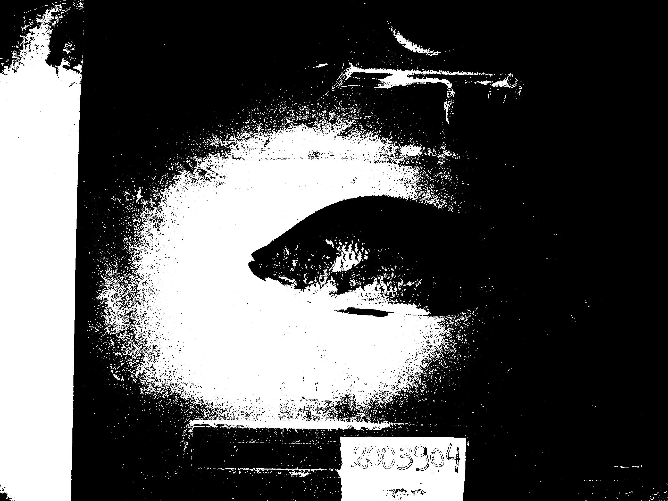
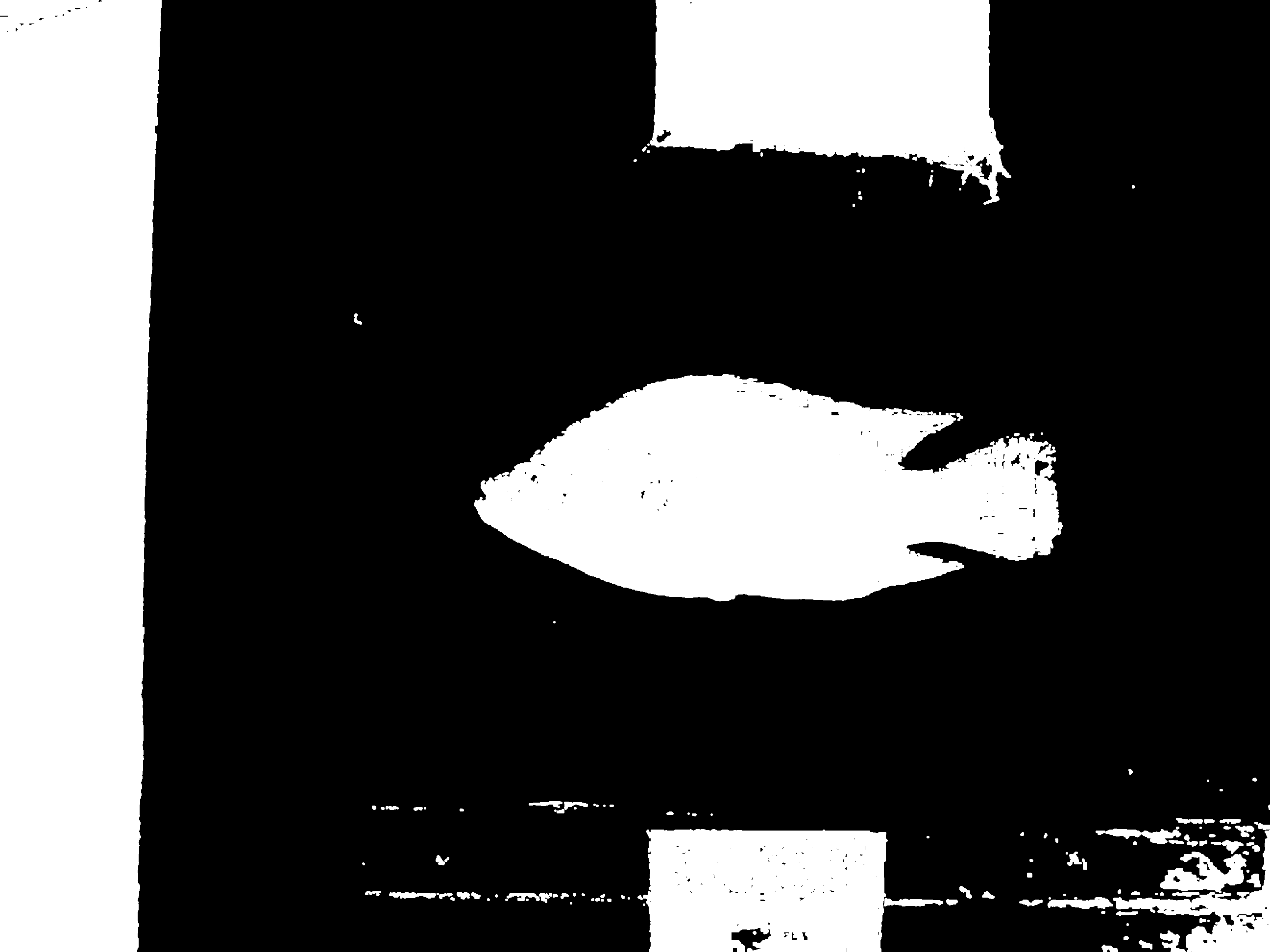
4. Mask fusion and morphological cleanup

This is the point where the full pipeline becomes more reliable than the earlier one-channel attempts. The saturation and brightness evidence are merged first, then restricted so that only regions compatible with the hue prior survive. After that, morphological cleanup removes small mask noise and repairs cracks so the fish body becomes a more stable connected shape. The result is then inverted to make the remaining background-connected structures easier to reject in the next stage.

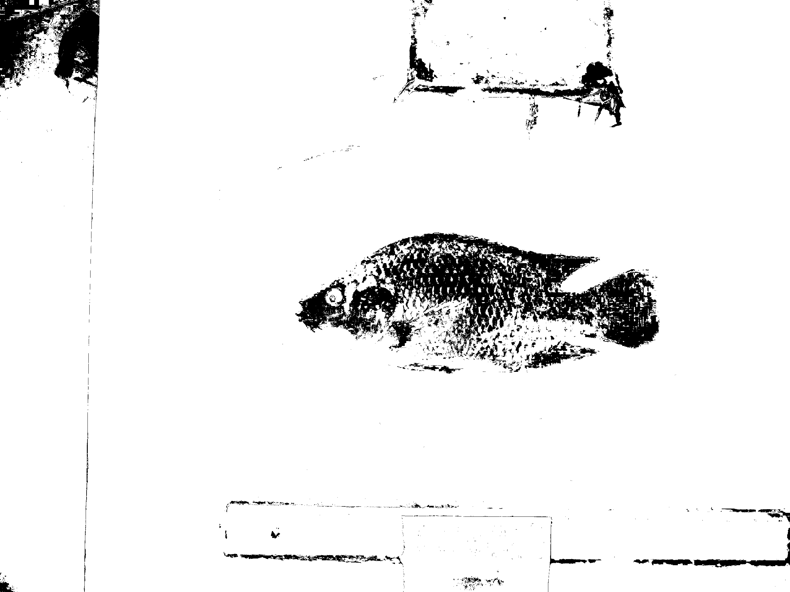
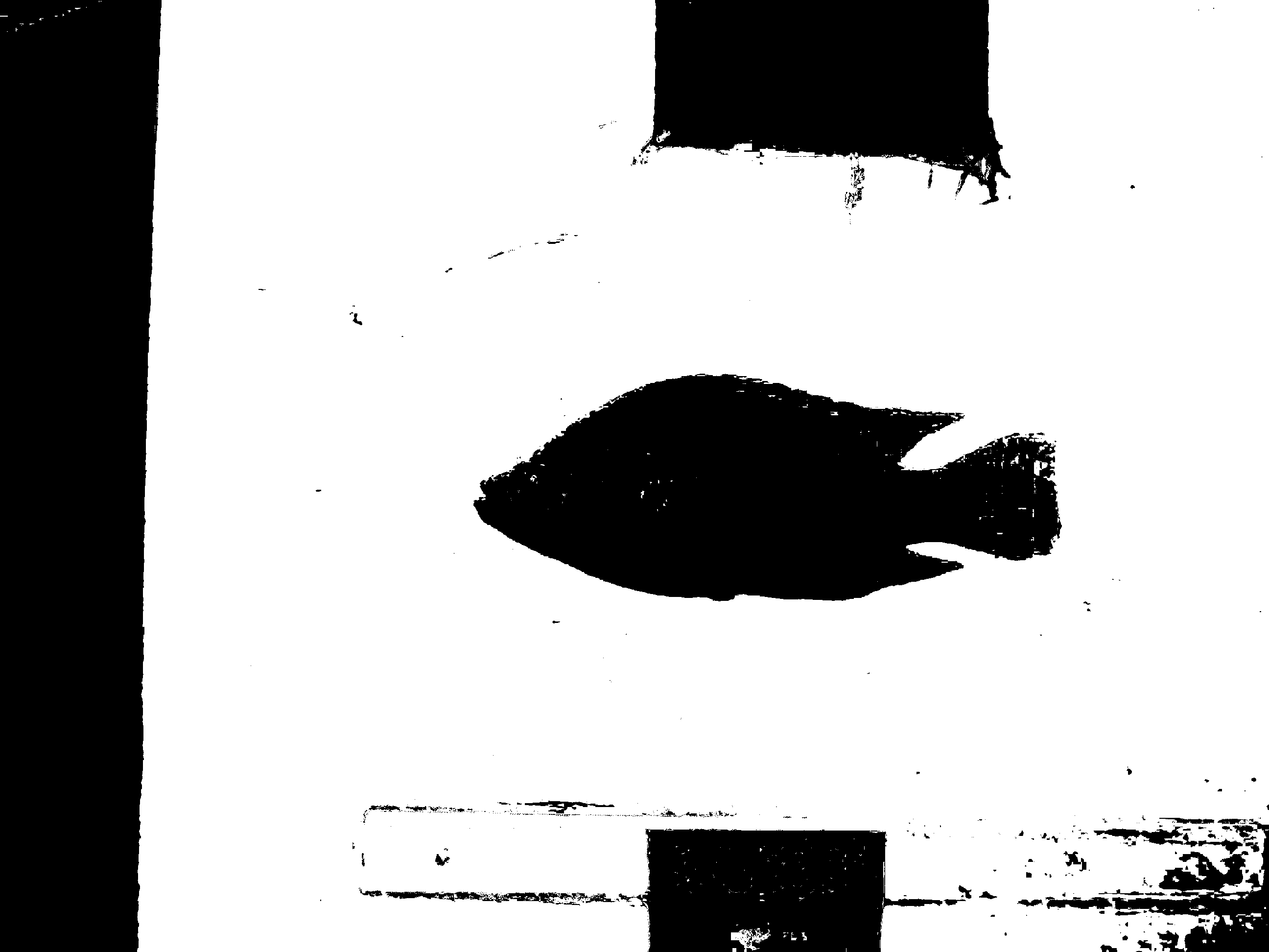
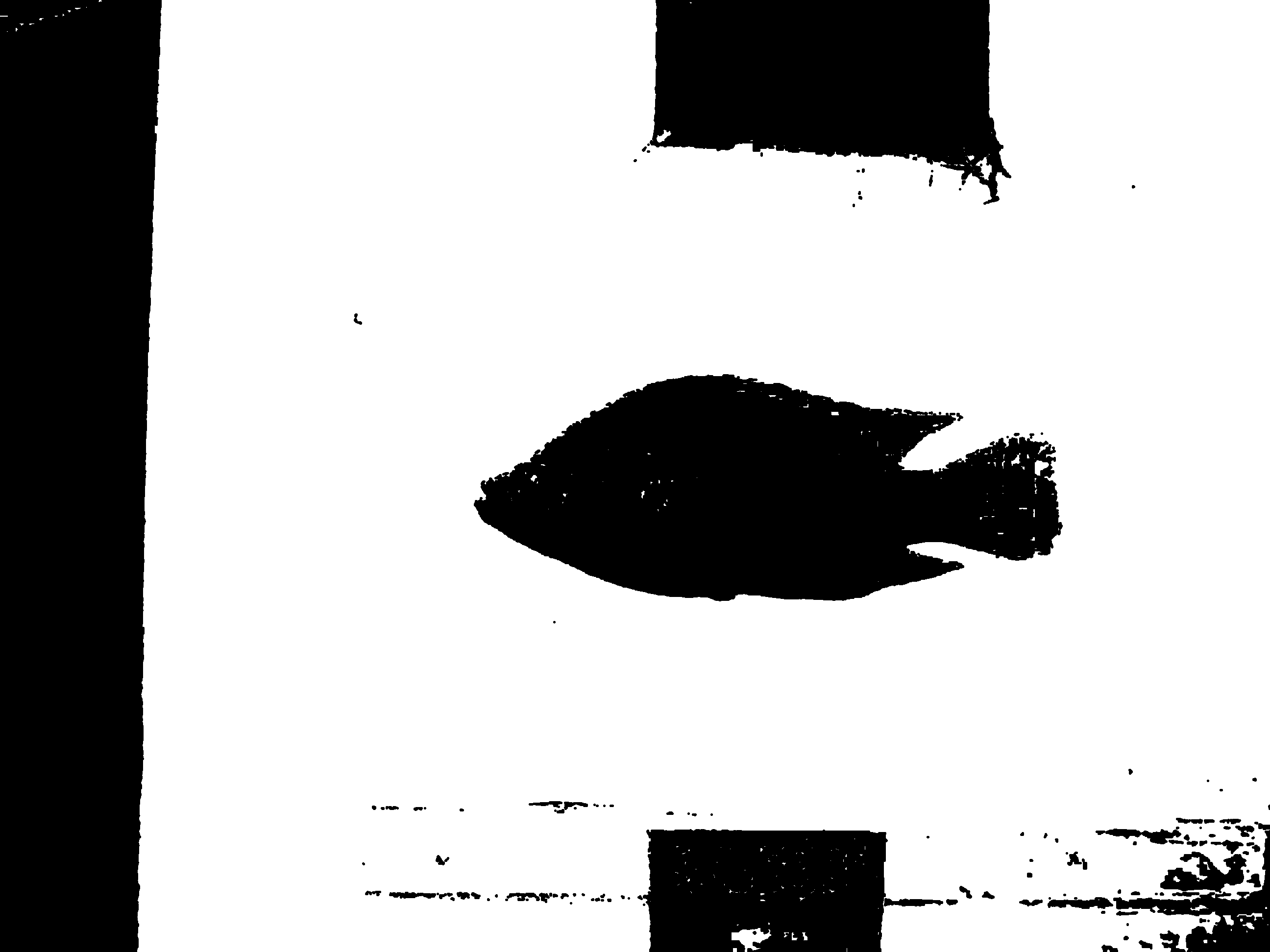
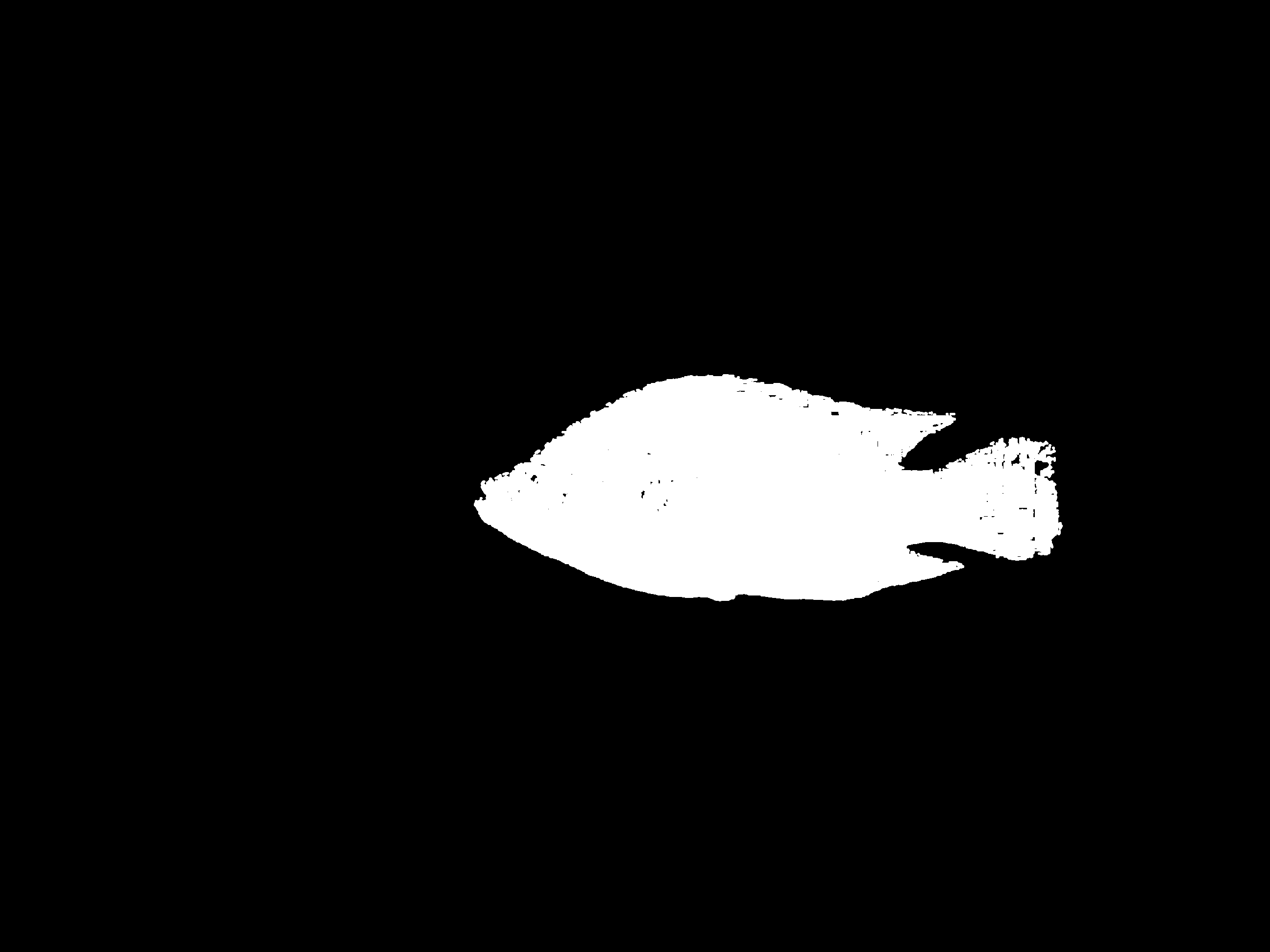
5. Component selection and final mask

At this stage the fish is mostly isolated, but a few leftover regions still need to be removed. The main rule here is structural rather than purely photometric: anything still touching the image boundary is unlikely to be the fish. The pipeline therefore keeps the dominant interior component, converts that into the candidate fish region, and then fills remaining holes so the silhouette is suitable for downstream measurements.

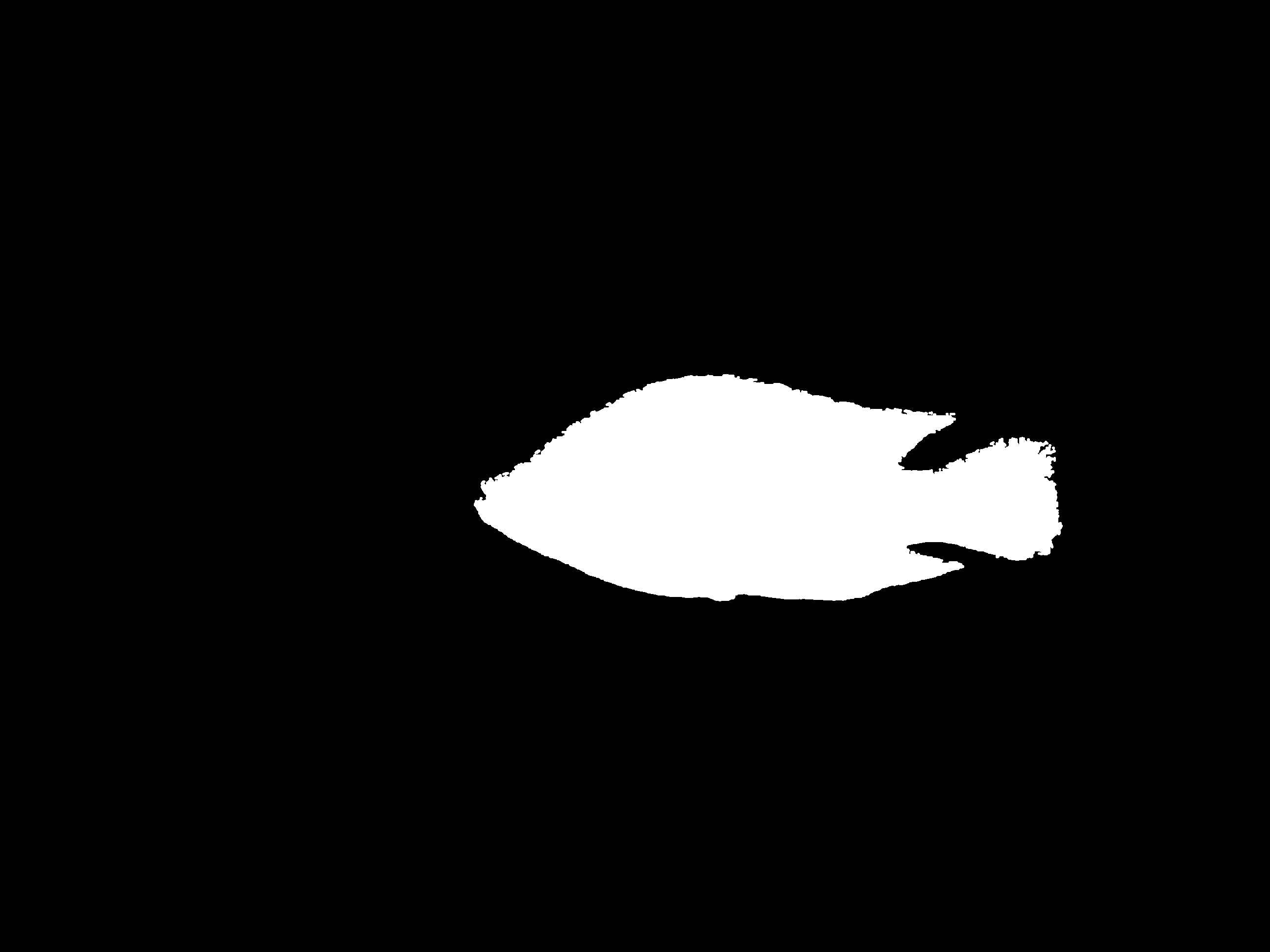
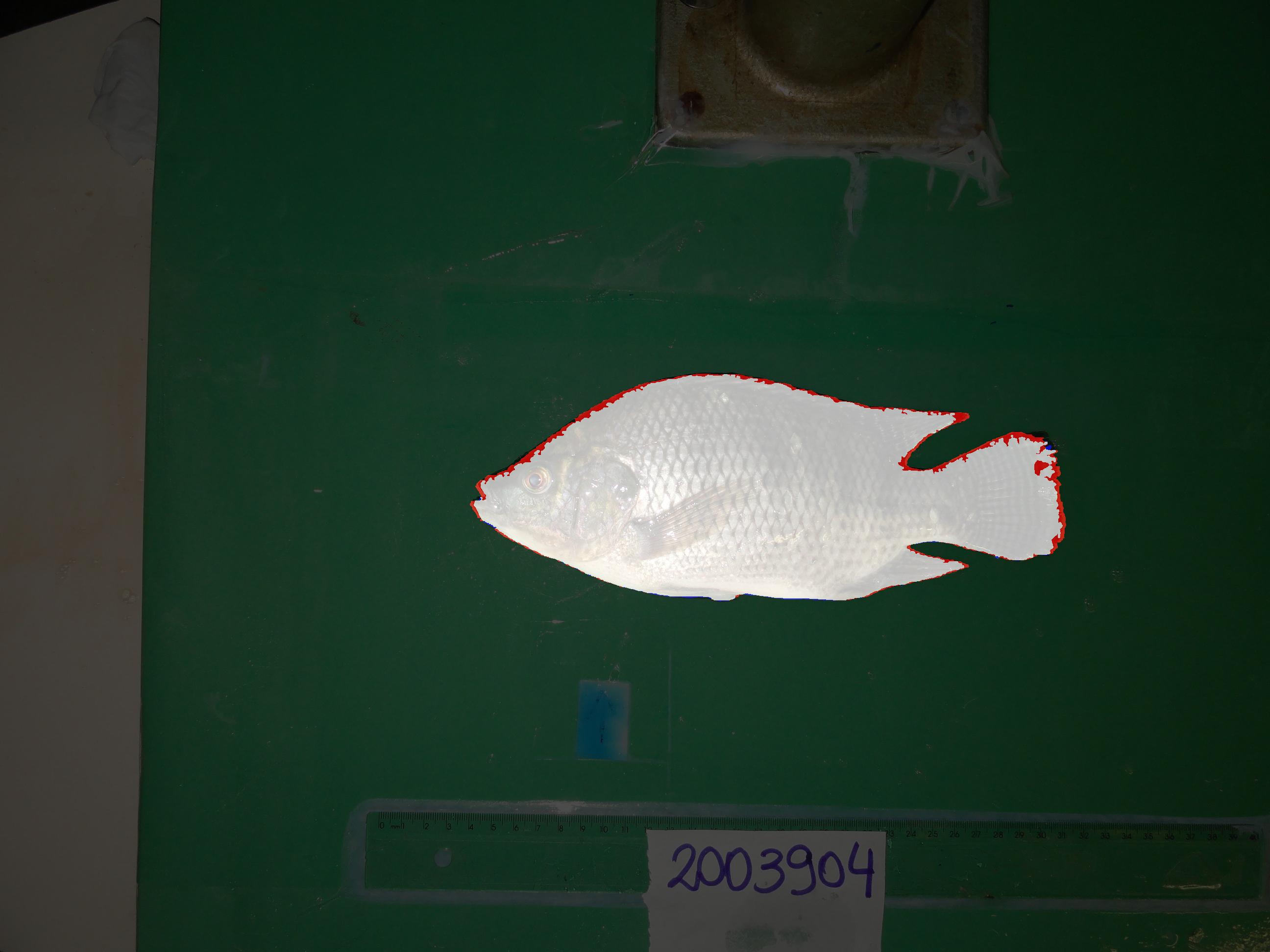
6. Prediction versus reference

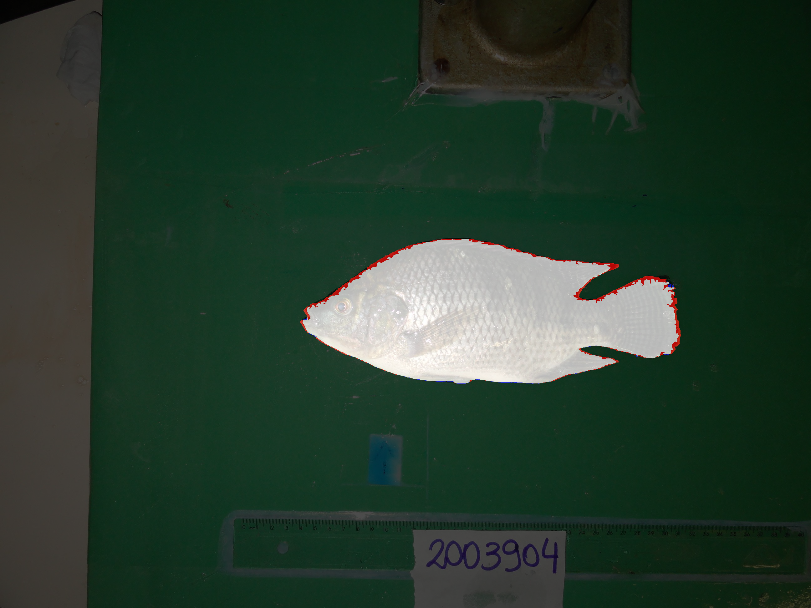
The final overlay compares the predicted mask with the reference mask for the same fish. White indicates agreement, red marks reference pixels the pipeline missed, and blue marks extra predicted pixels. For this sample, most of the boundary agrees, and the remaining disagreement is concentrated around fine contour details rather than catastrophic leakage into the board.

This walkthrough is the clearest representation of the project. It shows how the final algorithm turns one raw image into a usable segmentation through color decomposition, thresholding, fusion, morphology, and structure-aware component filtering.

Full algorithm

The complete implementation used for the final submission is included below for reference.

findFishGS[img_] := Module[{},
	{himg, simg, bimg} = ColorSeparate[img, "HSB"];
	hBinImg = Binarize[himg, {0.35, 0.6}];
	sBinImg = Binarize[simg, {0.25, 1}];
	bBinImg = Binarize[bimg, {0.7, 1}];
	sb = ImageAdd[sBinImg, bBinImg];
	hsb = ImageMultiply[hBinImg, sb];
	aa = Closing[hsb, DiskMatrix[2]];
	bb = ColorNegate[aa];
	sizes = ComponentMeasurements[
		bb,
		{"Area", "AdjacentBorderCount"},
		(#1 > 1000 && #2 == 0) &
	];
	If[Length[sizes] == 0, Print[img]];
	maxKeys = Keys[MaximalBy[sizes, #[[2]] &]];
	masktemp = Image[
		ComponentMeasurements[bb, "Mask"][[maxKeys, 2]][[1]]
	];
	mask = FillingTransform[masktemp];
	{mask, extractParams[mask]}
]

Evaluation examples

After the pipeline was stable on representative samples, I ran it across a broader set of fish images and kept several overlays from that evaluation pass. Those examples are more useful than a single success case because they show how the same handcrafted pipeline behaves across different fish sizes, poses, and lighting conditions.

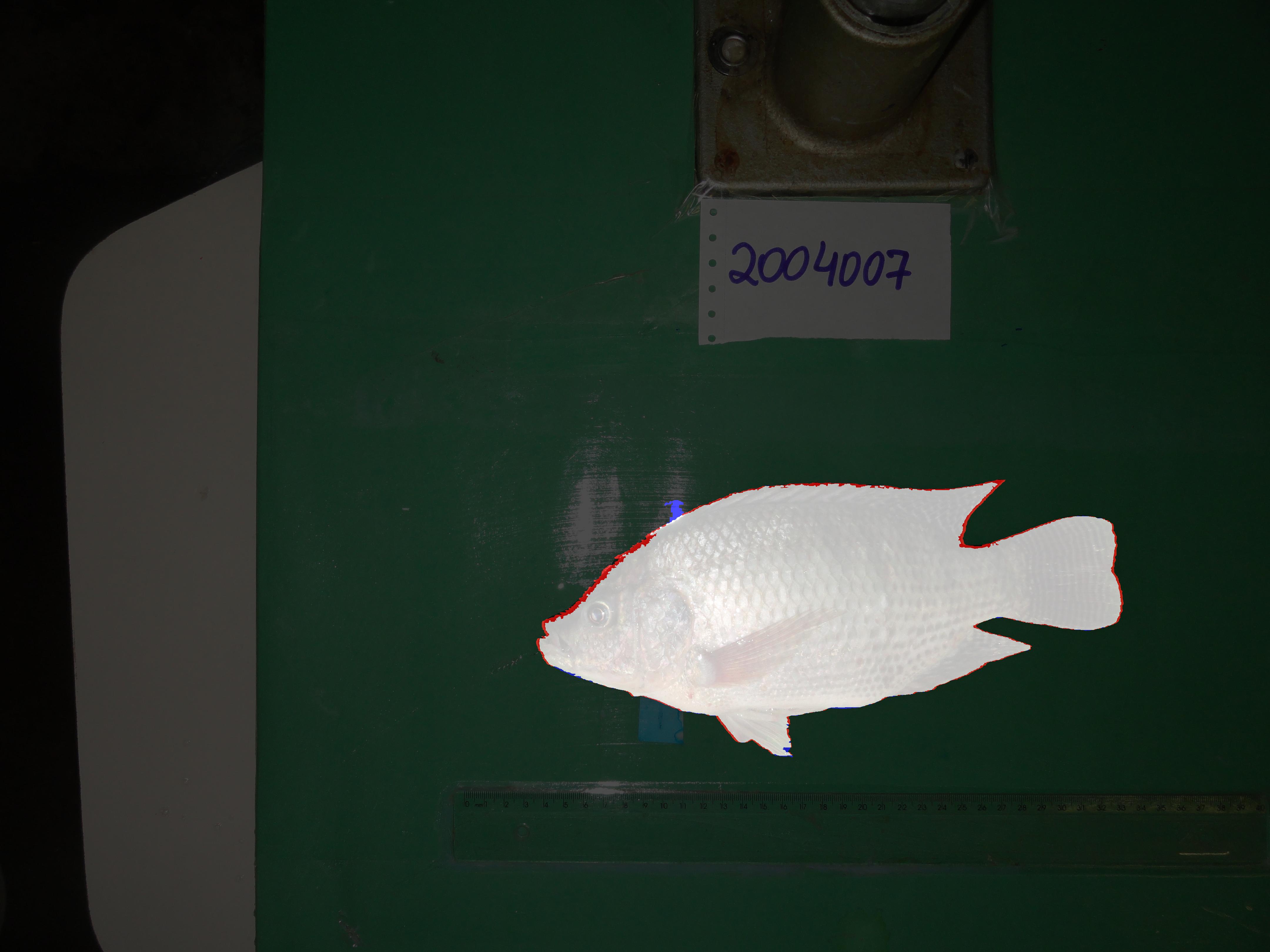
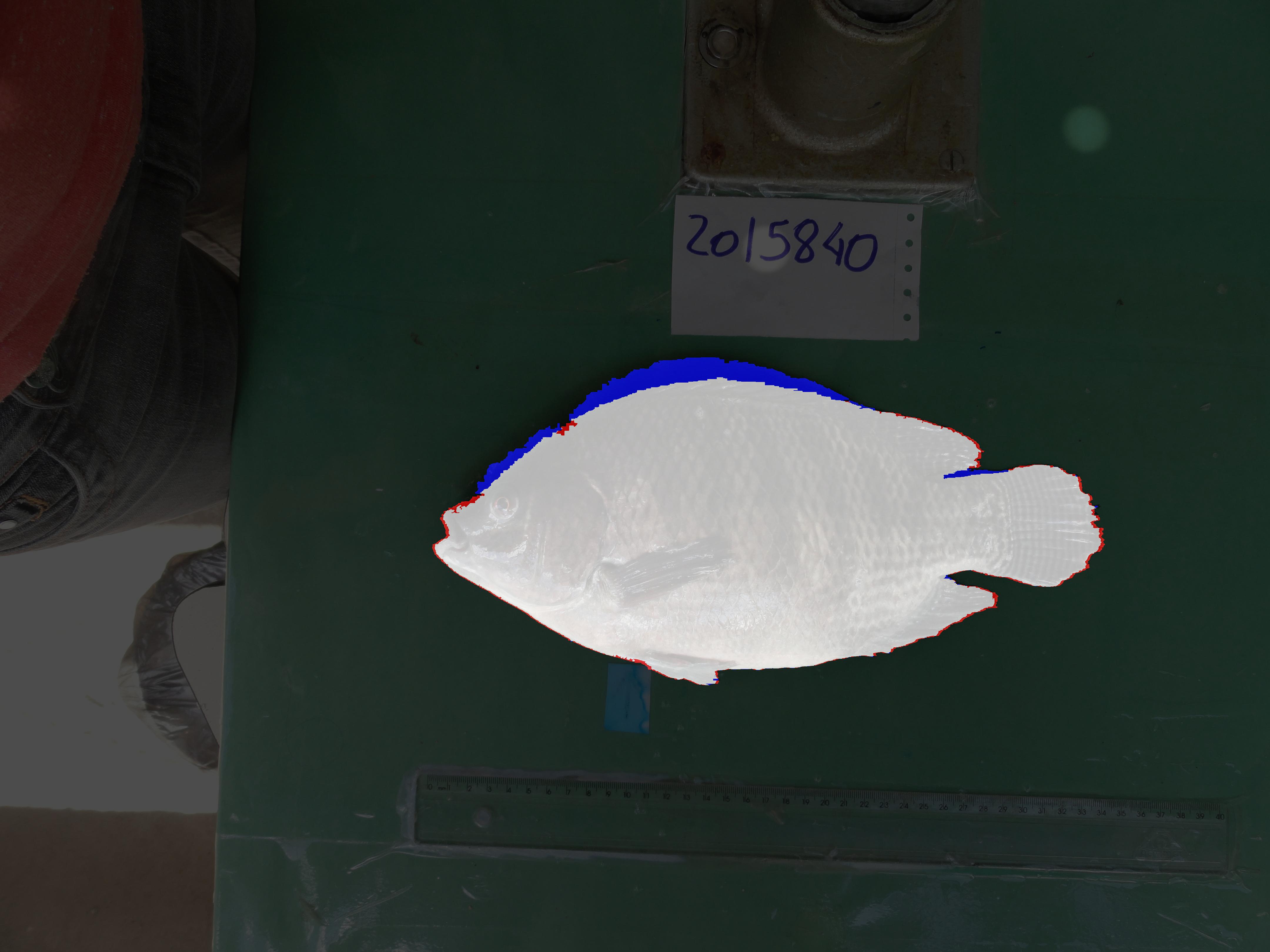
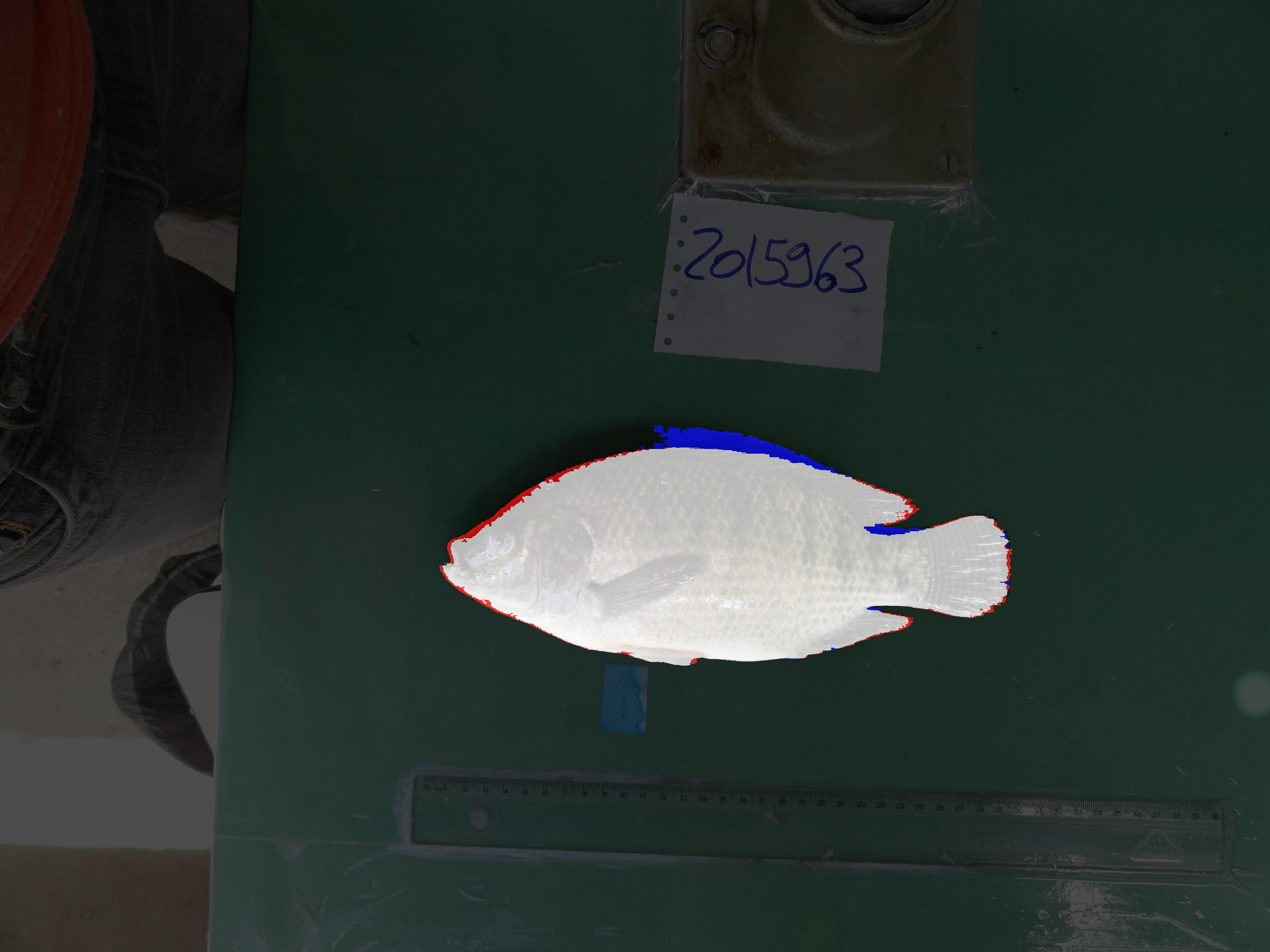
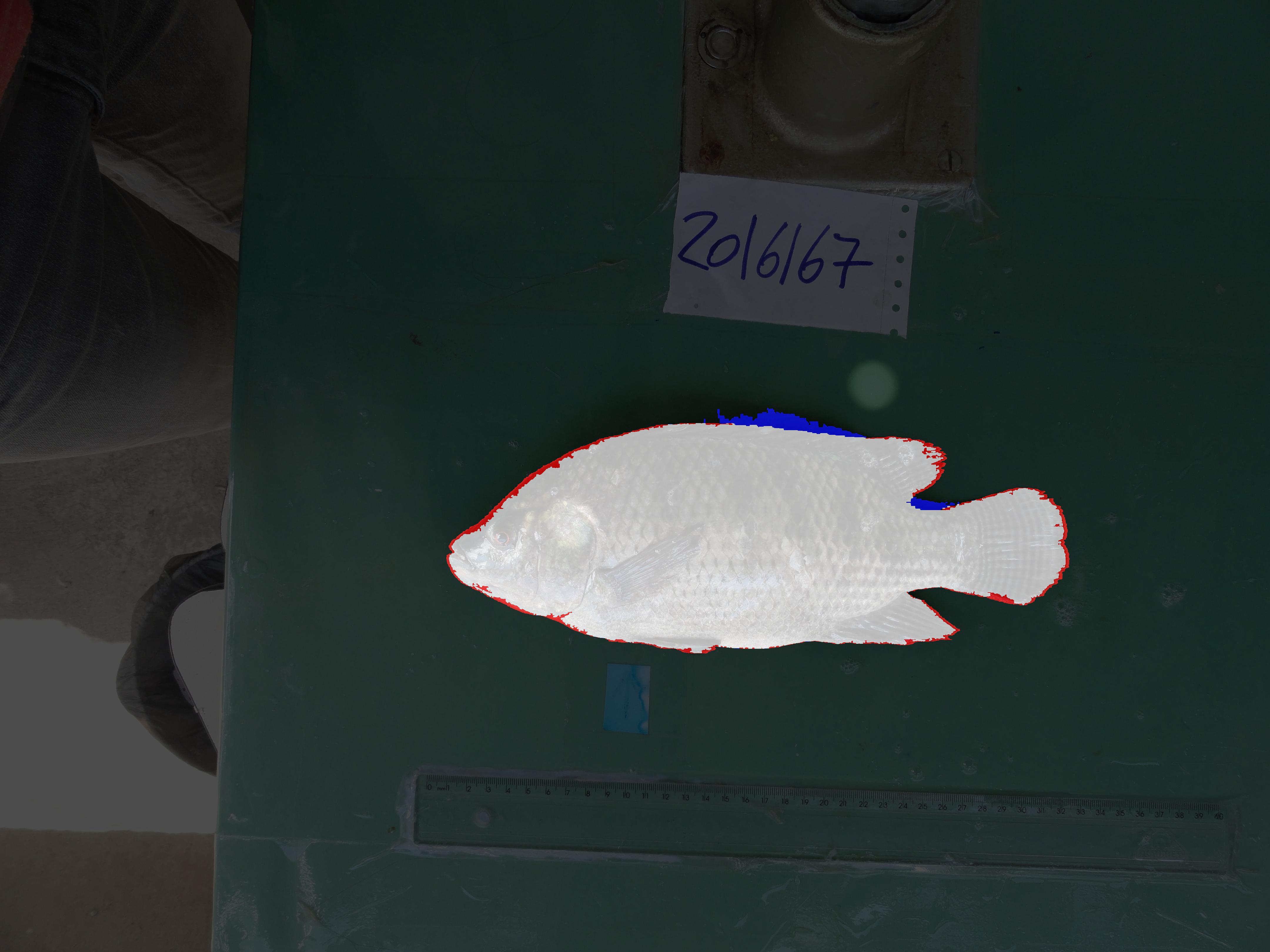
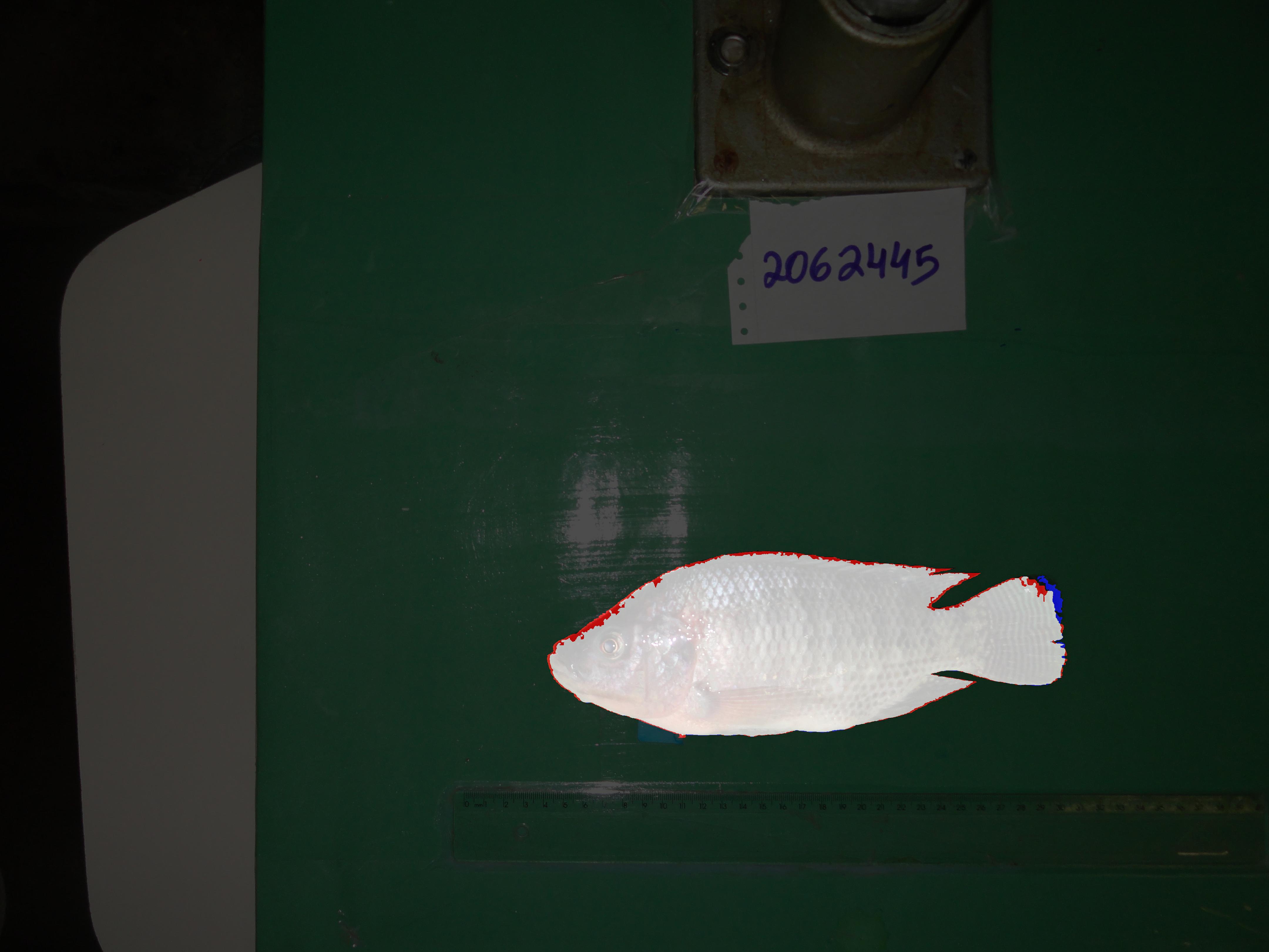
What stands out in these results is that the silhouette stays stable across size changes, pose changes, and moderate lighting differences. When errors do appear, they are usually concentrated along fine upper-boundary regions, which is exactly the kind of behavior you would expect from a handcrafted threshold-and-morphology pipeline.

Why the approach worked

From a machine learning perspective, the strength of this project is that the final solution is still fairly interpretable. It does not rely on a learned model or a large feature-engineering stack. Instead, it uses a sequence of decisions that line up closely with the image statistics of the task:

1. the board is mostly green,
2. reflective regions are bright but do not behave like the fish across all three HSB channels,
3. false positives often connect to the border,
4. and the fish region should become a single dominant interior component after cleanup.

What I learned

This project made the strengths and limits of algorithmic vision methods much clearer to me. In a constrained environment with a strong prior, a carefully designed programmatic pipeline can produce plausible results without any training data at all. At the same time, every uncontrolled variable becomes critical to performance. Reflections, lighting direction, shadows, and general photo conditions all have to be treated correctly, and handling those factors ends up being the hard part of the system.

It also made the tradeoff with data-driven methods much more concrete. A neural approach can often be more robust because it learns to absorb many of these variations from data, but that robustness comes at the cost of dataset collection, training time, and much heavier computation. Working through this project gave me a better sense of where algorithmic approaches are still effective, where they become fragile, and why that boundary matters in vision problems.