Juno Meets Jupiter: Recreating and Reimagining JunoCam Imagery

EEE 533

Overview

This project focused on reconstructing and reinterpreting raw JunoCam images of Jupiter. The work naturally split into two parts. In the first half, the goal was to match existing enhanced renderings from raw JunoCam image sets as closely as possible. In the second half, the same raw material was used more freely to create stylized but still structurally informative views of Jupiter’s atmosphere.

What made the project interesting is that the same raw spacecraft data supports both scientific reconstruction and expressive visualization. The first half is an optimization-driven reconstruction problem, while the second half is a visualization problem centered on making atmospheric structure legible.

Matching existing enhancements

For image sets 1 to 3, I treated enhancement matching as a reverse-engineering problem. The main assumption was that the target image could be approximated by fitting each channel separately and then recombining the result. That assumption works surprisingly well for the first two cases and gets close on the third, but it is also where the limitations of the approach become visible.

Set 1

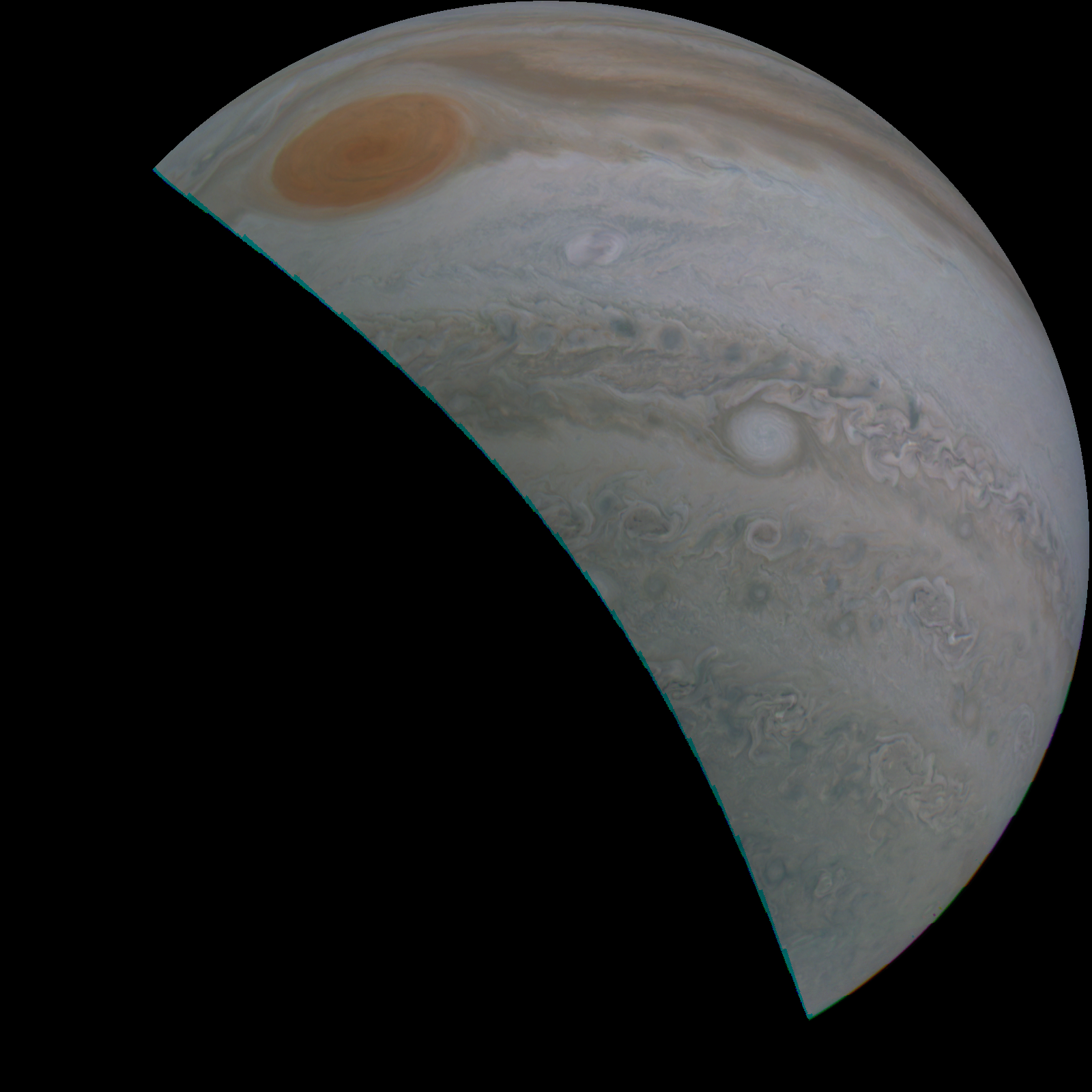
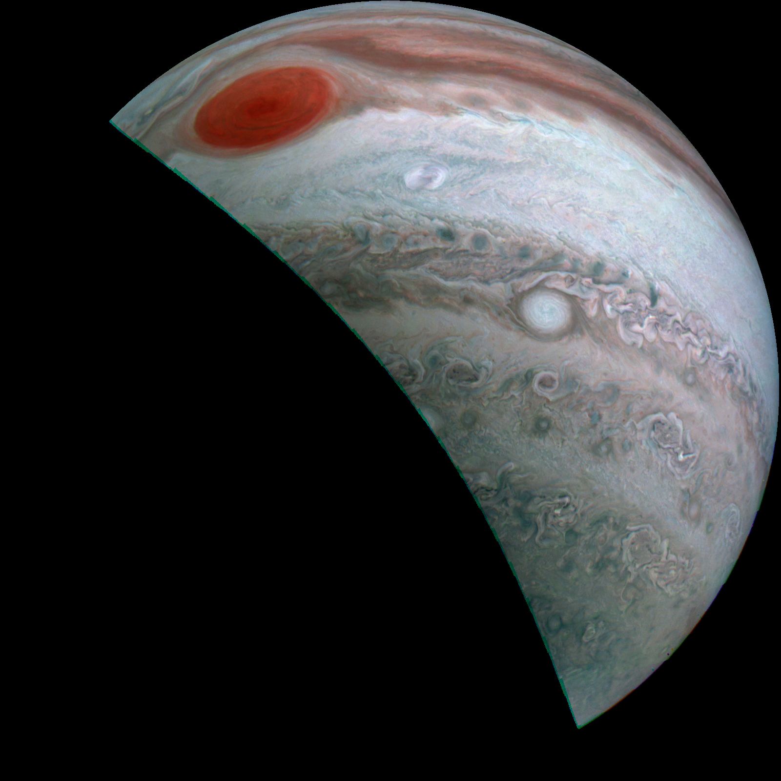
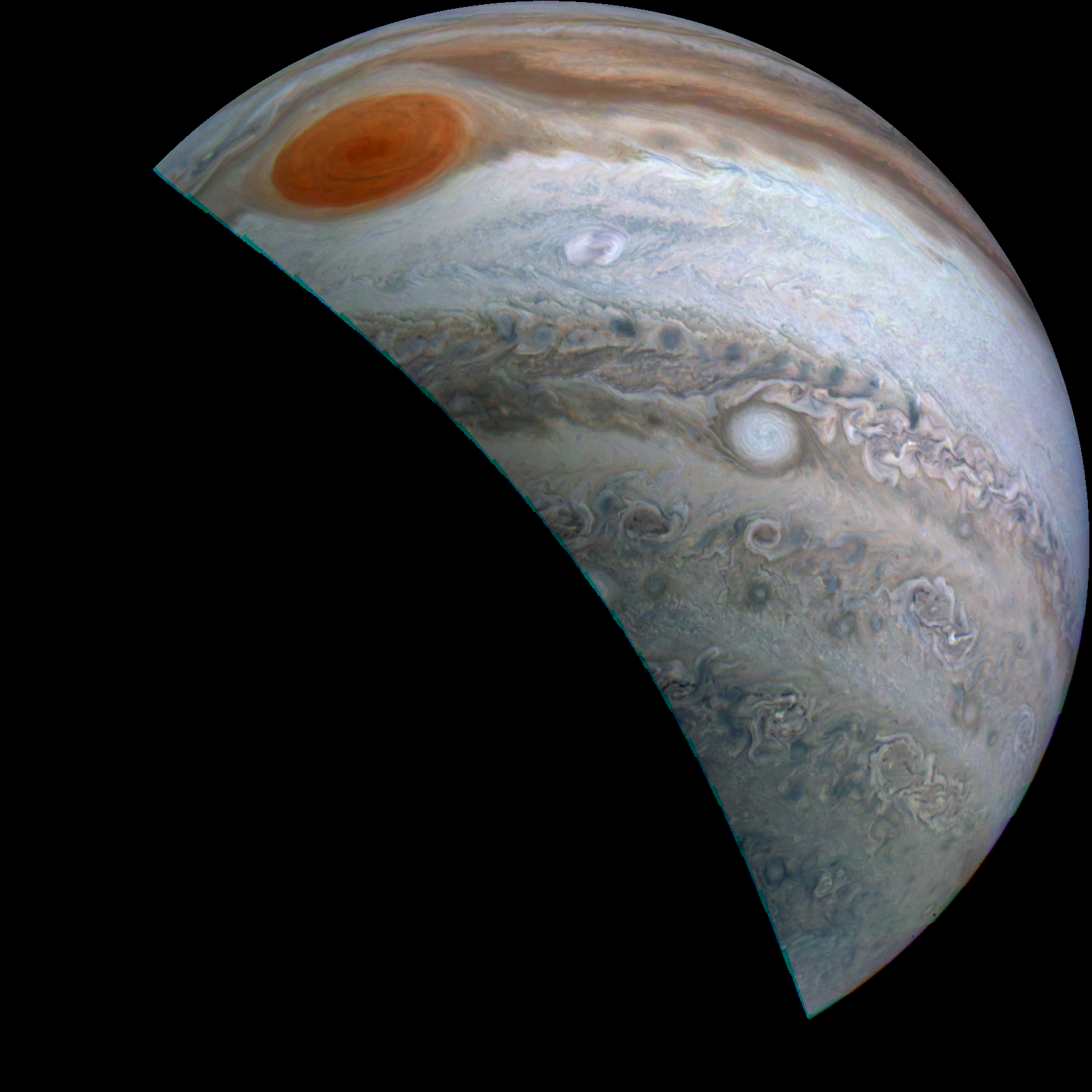
For the first set, I started with the simplest possible reverse-engineering idea: treat the target enhancement as the result of separate channel remapping and solve for the parameters that make each reconstructed channel as close as possible to the target. This produces a strong first match and establishes the basic pipeline used for the rest of the reconstruction section.

findoptchan[pc_,oc_]:=Module[{c, b, r, optparam, loss},
loss[{c_?NumericQ, b_?NumericQ, r_?NumericQ}]:=Module[{adjusted, subtracted, diff},
adjusted = ImageAdjust[pc, {c, b, r}];
subtracted = ImageData[adjusted]-ImageData[oc];
diff = Norm[Flatten[subtracted]];
diff
];
optparam=NMinimize[{loss[{c,b,r}], -1<c<=2, -1<b<=2, 0<r<=2},{c, b, r}];
optparam
];

loss[{c_, b_, r_}] := Norm @ Flatten[
  ImageData[ImageAdjust[pc, {c, b, r}]] - ImageData[oc]
];

rparam = findoptchan[pr, or];
gparam = findoptchan[pg, og];
bparam = findoptchan[pb, ob];

enhanced = ColorCombine[{
  ImageAdjust[pr, Values[rparam[[2]]]],
  ImageAdjust[pg, Values[gparam[[2]]]],
  ImageAdjust[pb, Values[bparam[[2]]]]
}, "RGB"];

Set 2

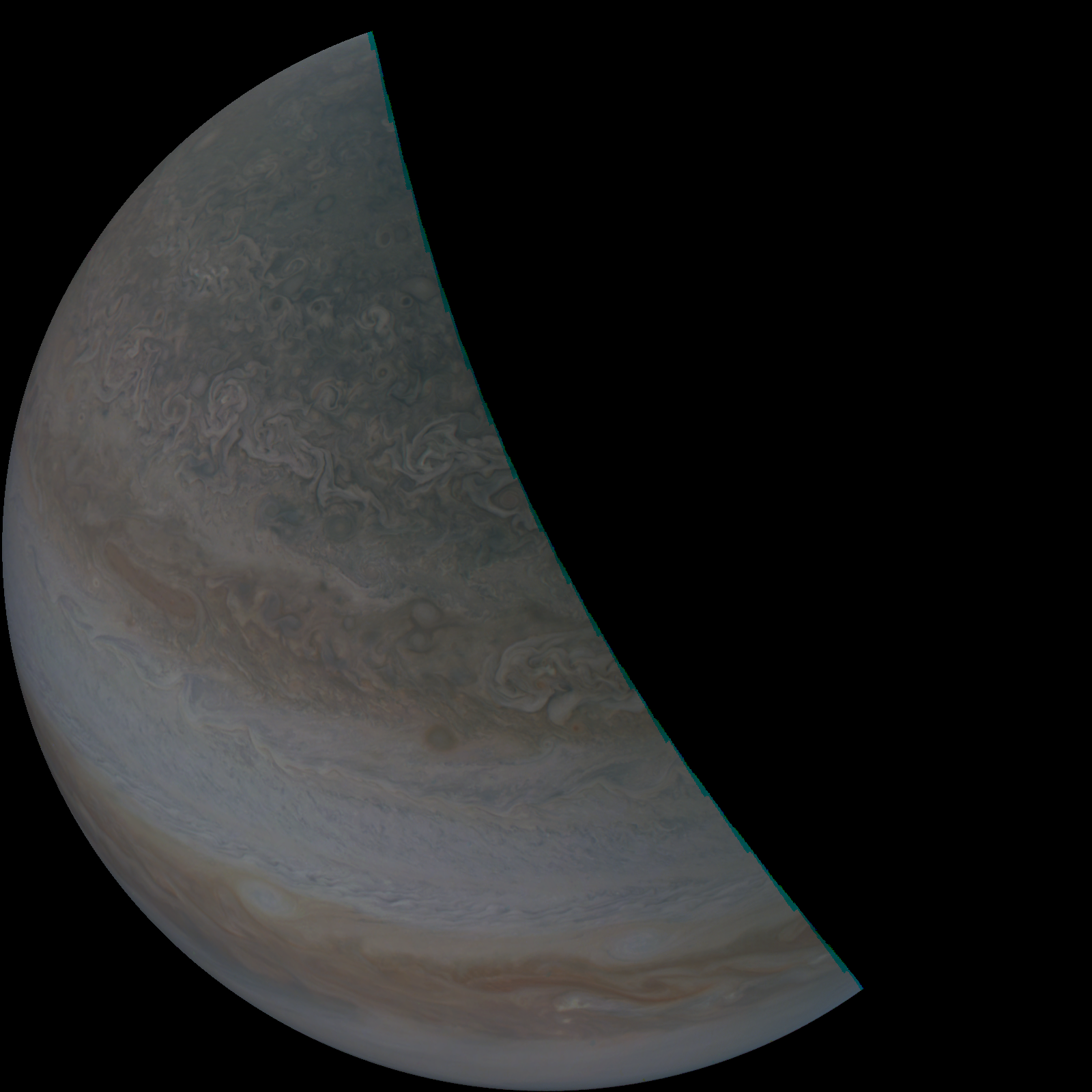
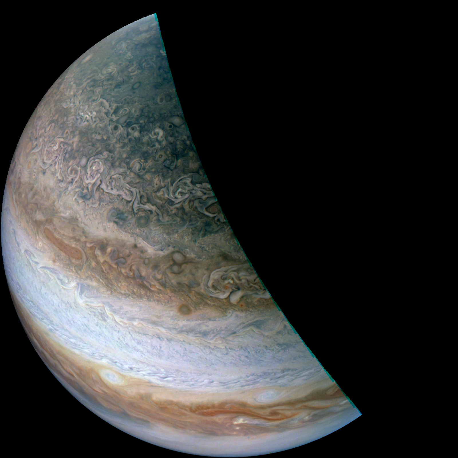
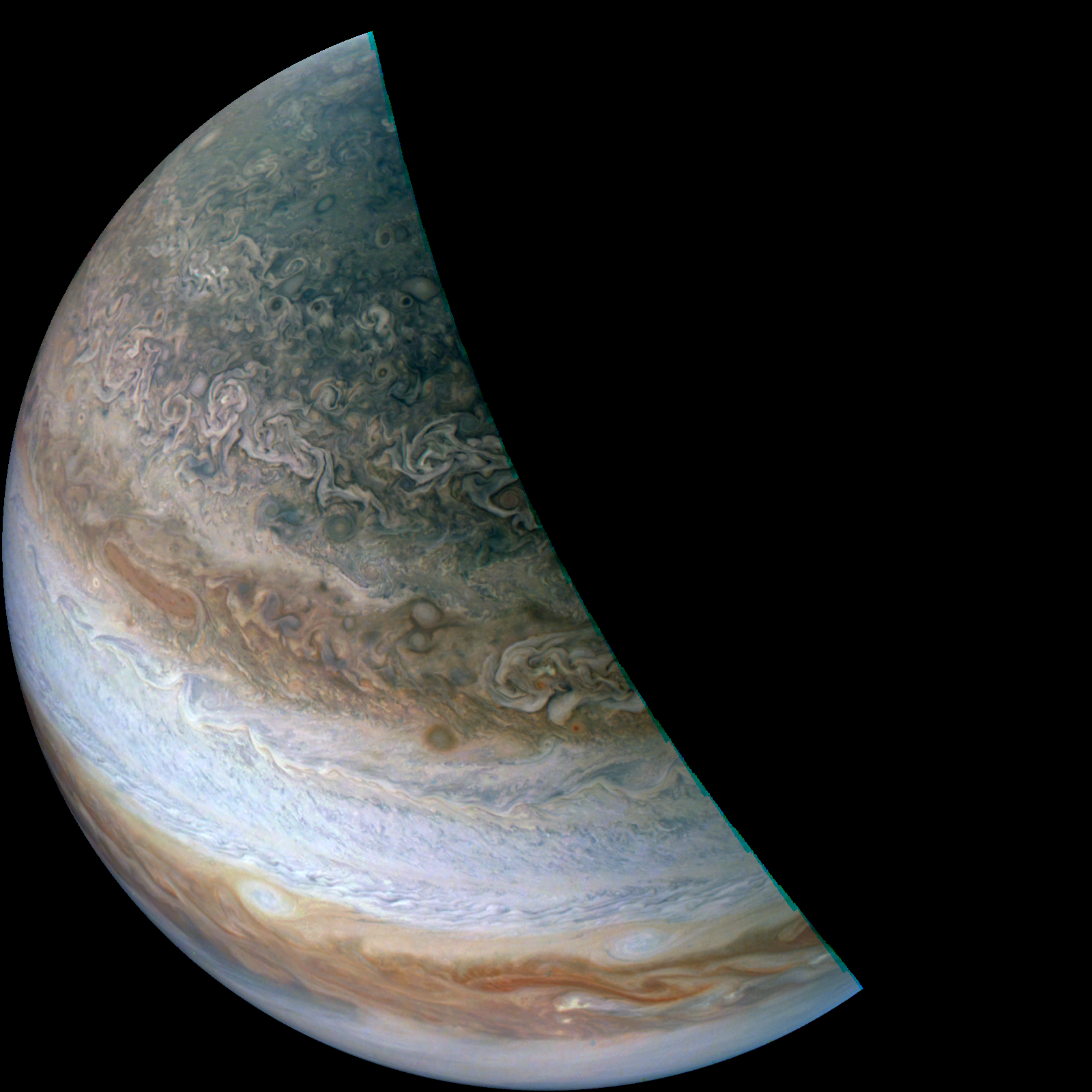
The second set is useful because it tests whether the same modeling assumption transfers to another image rather than only fitting one example. It does. The reconstructed result is still not a pixel-perfect clone, but it stays close enough to show that a channelwise model captures a large fraction of the original enhancement logic.

params2 = {
  Values[findoptchan[pr, or][[2]]],
  Values[findoptchan[pg, og][[2]]],
  Values[findoptchan[pb, ob][[2]]]
};

enhanced2 = ColorCombine[{
  ImageAdjust[pr, params2[[1]]],
  ImageAdjust[pg, params2[[2]]],
  ImageAdjust[pb, params2[[3]]]
}, "RGB"];

Set 3

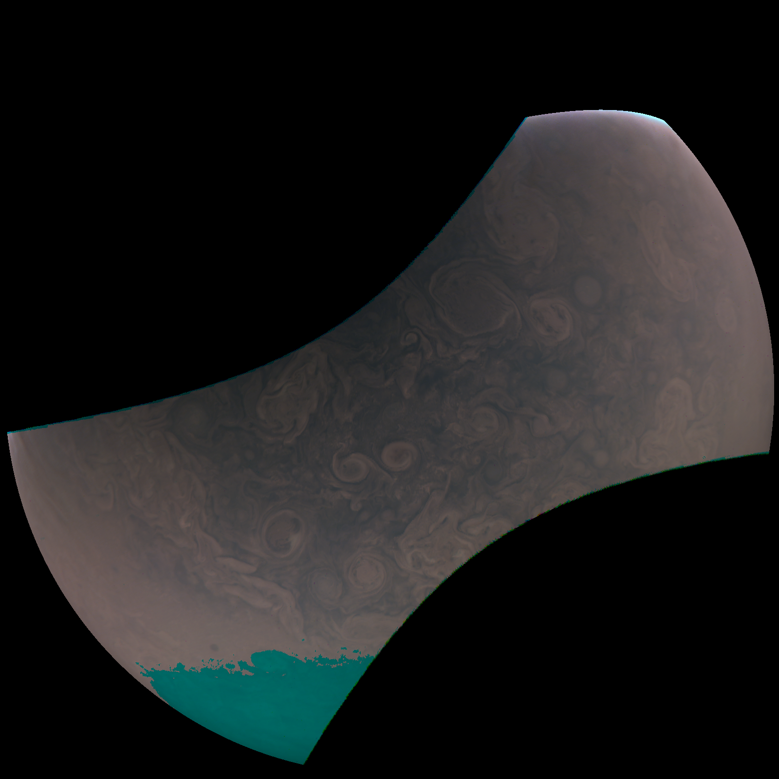
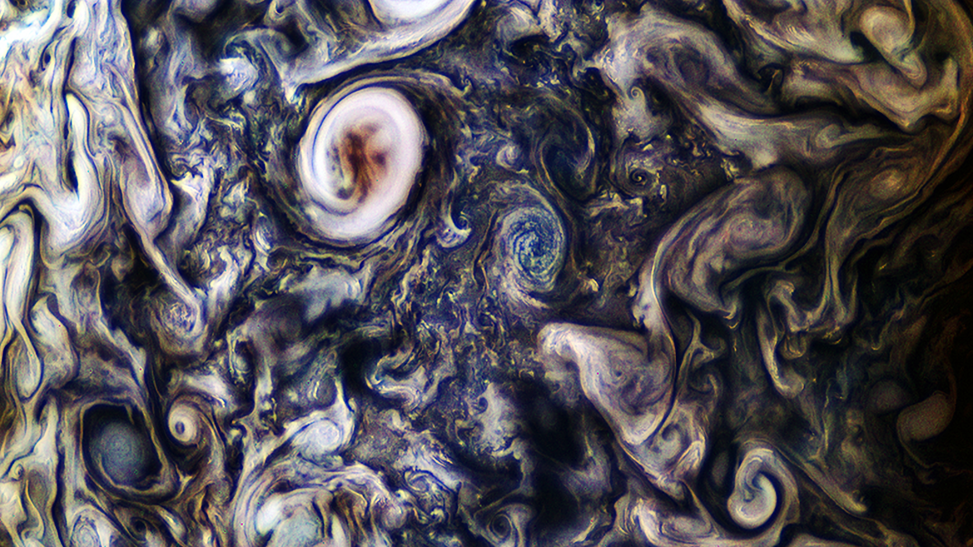
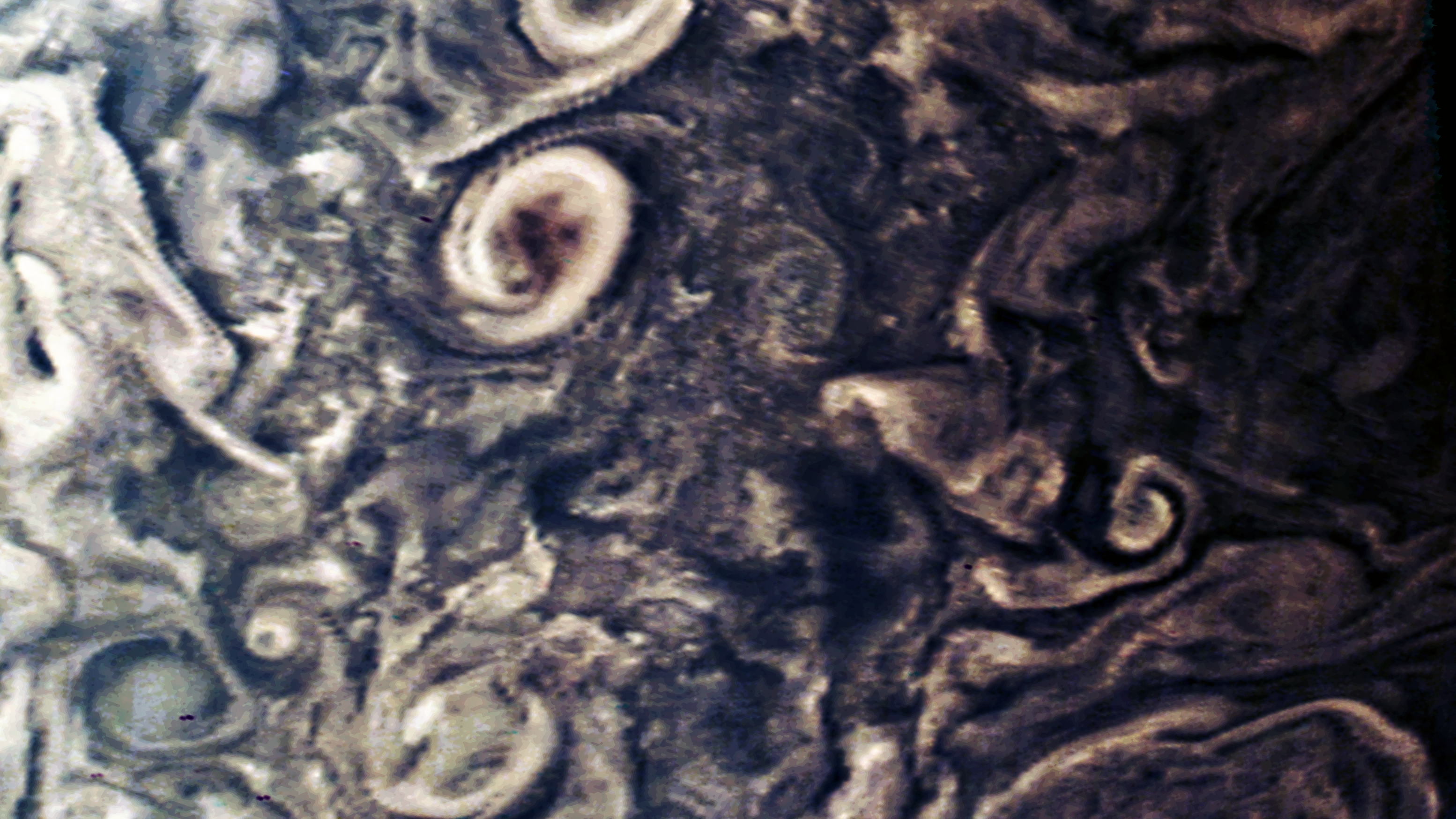
The third set is the point where the basic assumption starts to bend. A channelwise fit still gets the reconstruction in the right neighborhood, but additional alignment and post-processing are needed to approach the target more closely. Even then, the result is only approximate, which makes the limits of this style of reverse engineering much clearer.

aligned = ColorCombine[
  ColorSeparate[ImageAlign[o, p]][[1 ;; 3]],
  "RGB"
];

params3 = findopt1[aligned, o];

enhanced3 = HistogramTransform[
  ImageEffect[enhance[aligned, params3], {"DetailEnhancing"}],
  o
];

Artistic image sets 4, 5, and 6

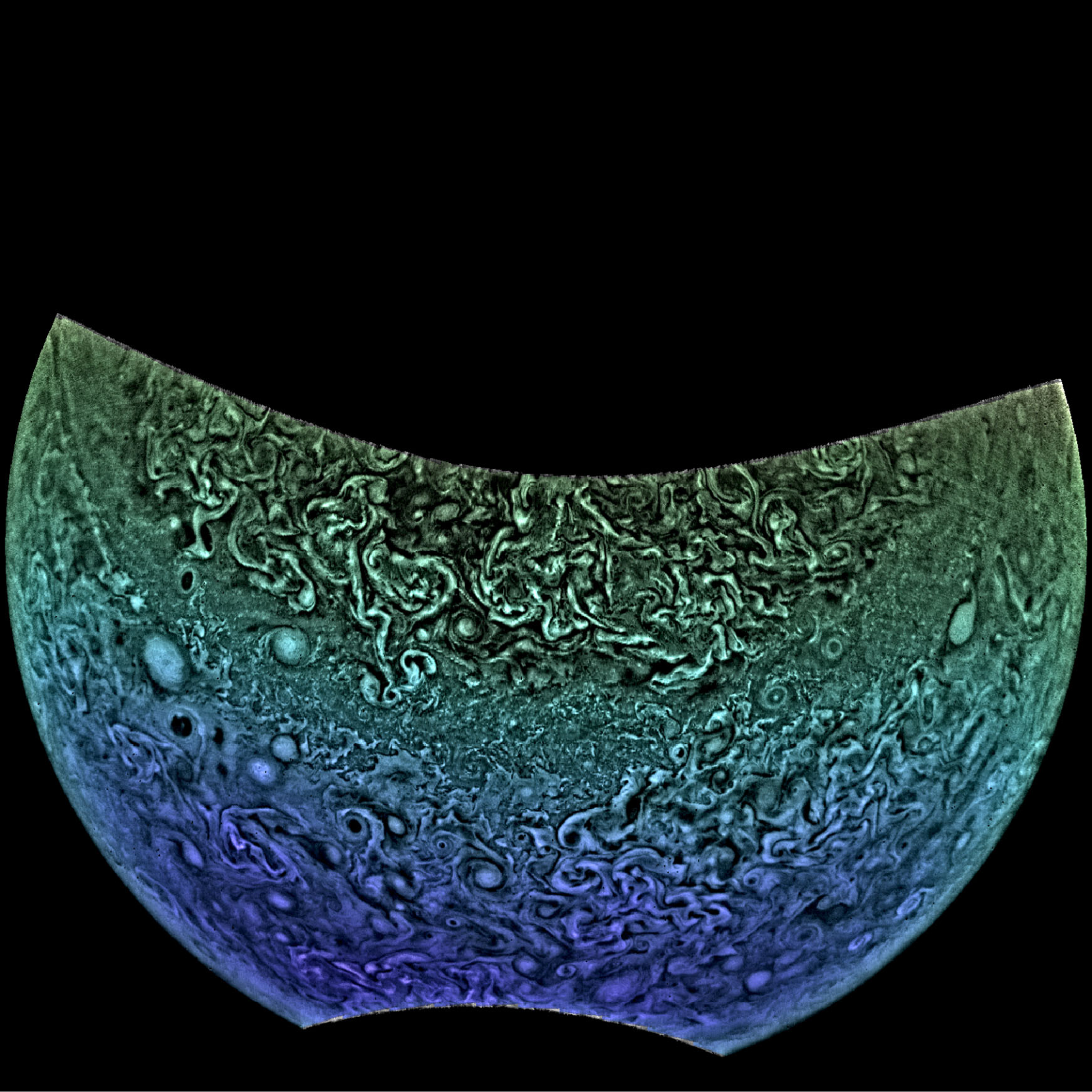
The second section shifts away from replication and toward exploration. For image sets 4 through 6, the emphasis is no longer on matching a reference exactly, but on applying transformations that make seams, textures, and atmospheric structure easier to notice.

Set 4

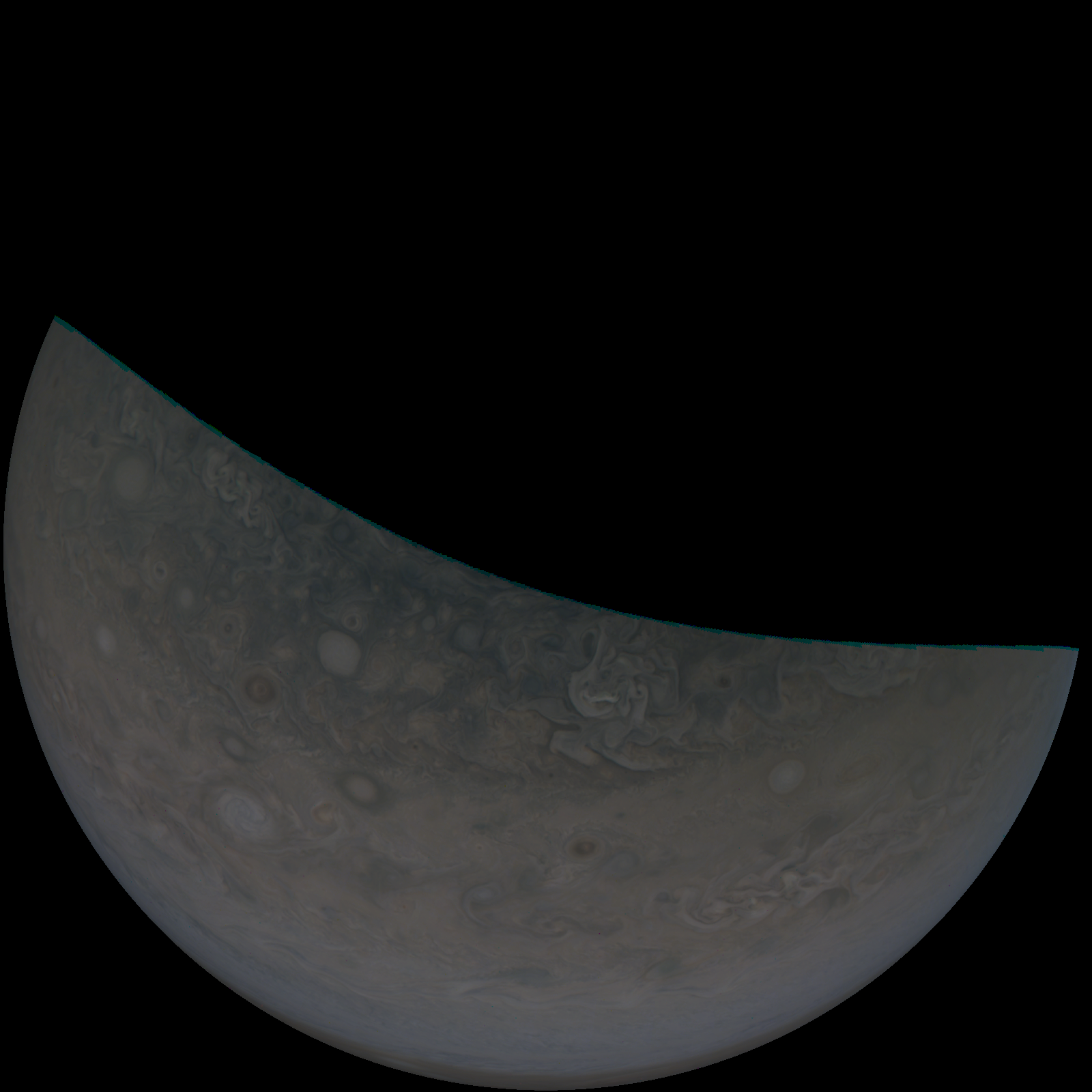
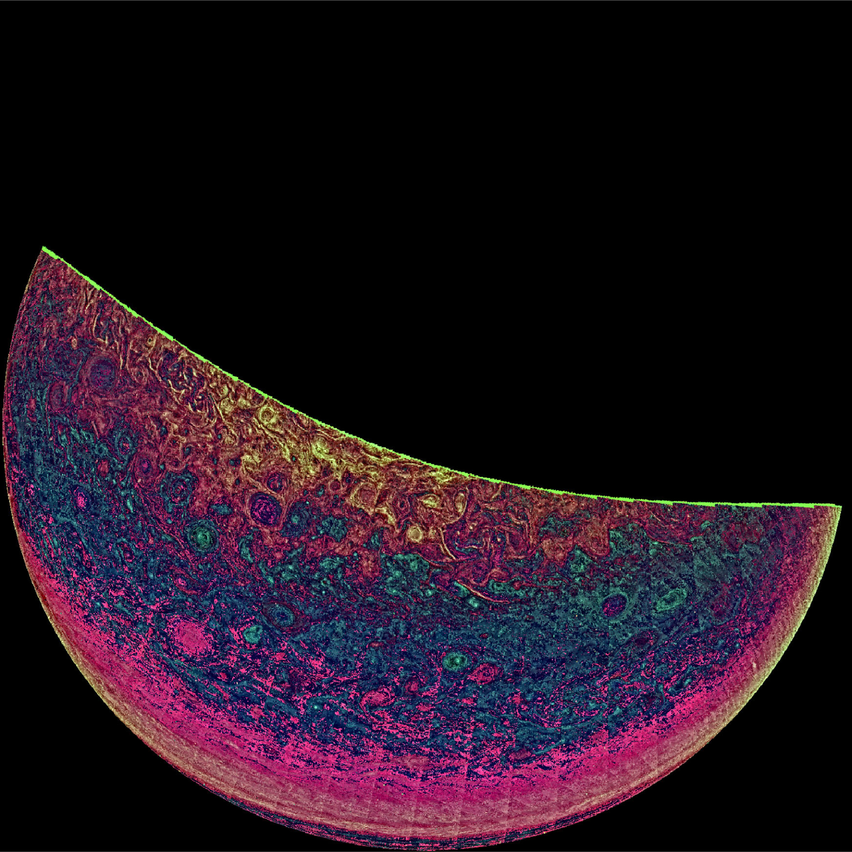
Set 4 was my first intentionally stylized rendering. I treated color as a design variable and pushed the image toward a more vivid, high-contrast planetary texture. That made the stitch lines and atmospheric transitions much more visible than they are in the original frame.

{hh, ss, bb} = ColorSeparate[p, "HSB"];

out = ColorCombine[{hh, ImageAdjust[ss] * 3, bb}, "RGB"];
out = ImageEffect[out, {"DetailEnhancing"}];
out = ImageAdjust[out];

Set 5

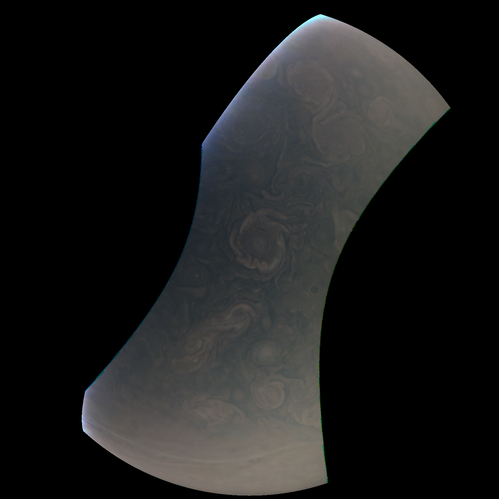
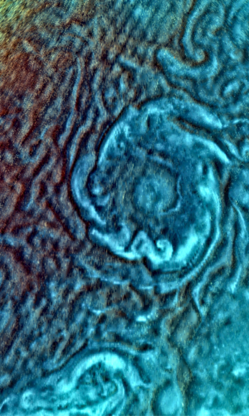
For set 5, I cropped into the storm eye and built the rendering around texture. The goal was to make the center feel sculpted rather than flat, so the enhancement layers a softened surface texture over a remapped color base. The result is less about faithful color and more about emphasizing the form of the storm.

p = ImageCrop[p, {300, 500}];
{r, g, b} = ColorSeparate[p, "RGB"];
{hh, ss, bb} = ColorSeparate[p, "HSB"];

out = ColorCombine[{ss, bb, r}, "RGB"];
emboss = ImageEffect[GaussianFilter[ss, 6], {"Embossing", 100, 0}];
out = ImageCompose[emboss, {out, 0.97}];
out = GaussianFilter[ImageEffect[ImageAdjust[out], {"DetailEnhancing"}], 1];

Set 6

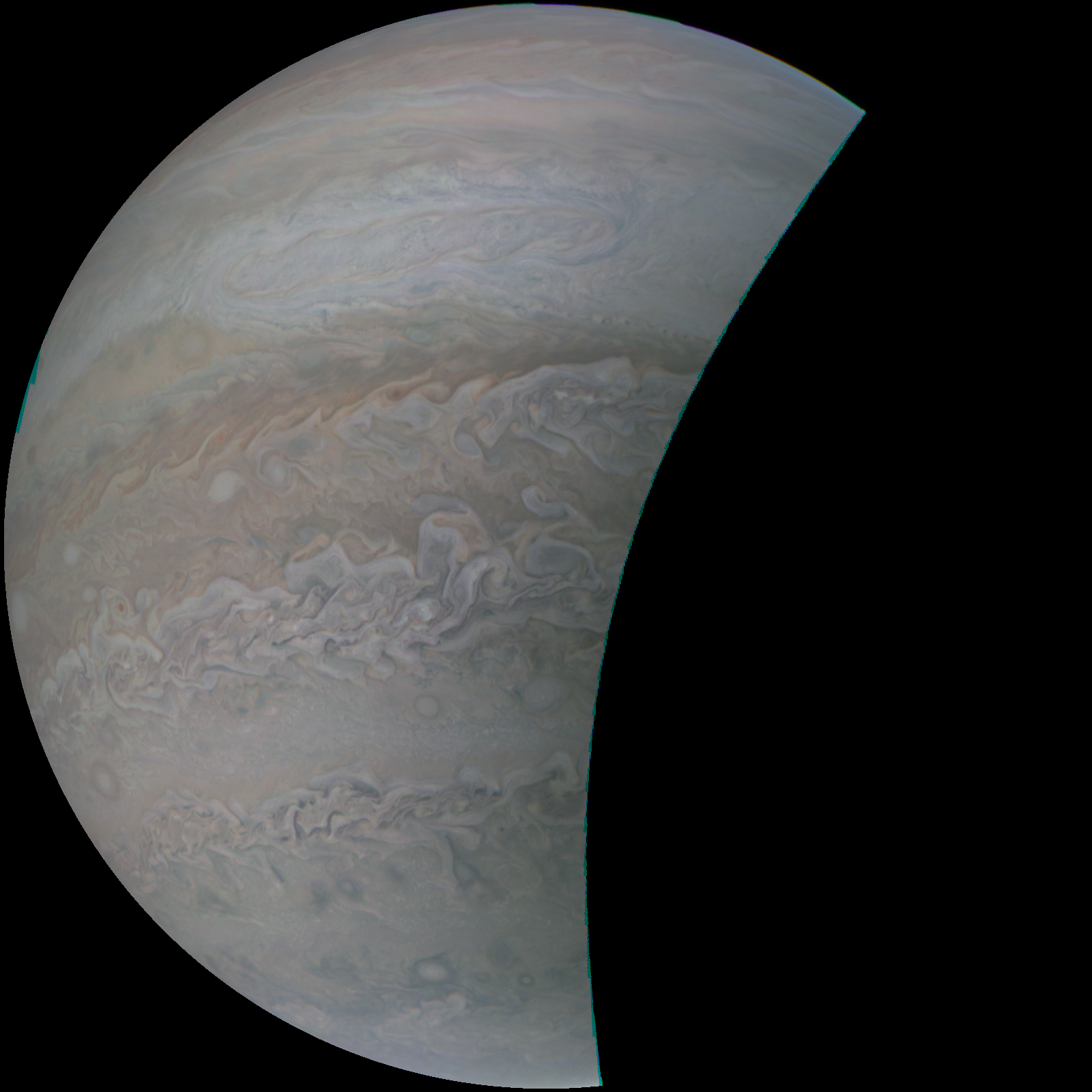
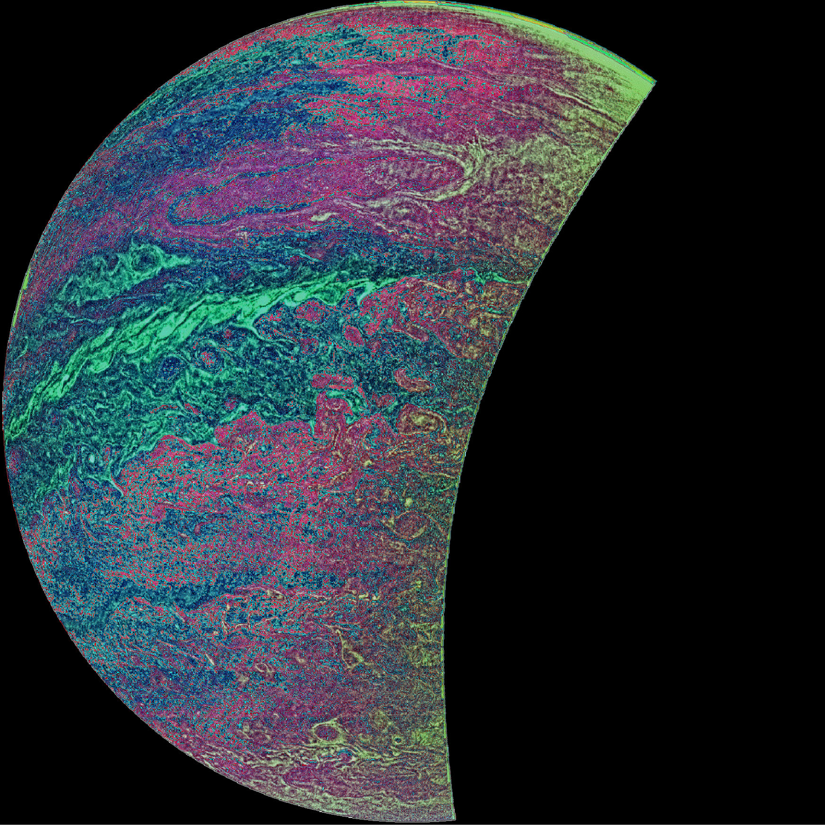
Set 6 keeps the same general color-remapping idea as set 4, but shifts the emphasis toward fine structure. I wanted the high-frequency ridges and folds to stand out more aggressively, so the rendering isolates that local structure and injects it back into the image as a separate visual layer.

{hh, ss, bb} = ColorSeparate[p, "HSB"];

out = ColorCombine[{hh, ImageAdjust[ss] * 6, bb}, "RGB"];
out = ImageAdjust[ImageEffect[out, {"DetailEnhancing"}]];

edgeh = LaplacianFilter[hh, 1];
edgeb = LaplacianFilter[bb, 1];
edgeimg = ColorCombine[{edgeb, edgeh, edgeh}, "RGB"];

out = ImageCompose[edgeimg, {out, 0.8}];
out = ImageAdd[out, edgeimg];

Personal JunoCam selections: sets 7, 8, and 9

The final section uses three additional JunoCam frames that I selected outside the original assignment sets. Here the processing becomes more personal and more visually bold, but the enhancements are still grounded in a specific structural idea from each image.

Set 7

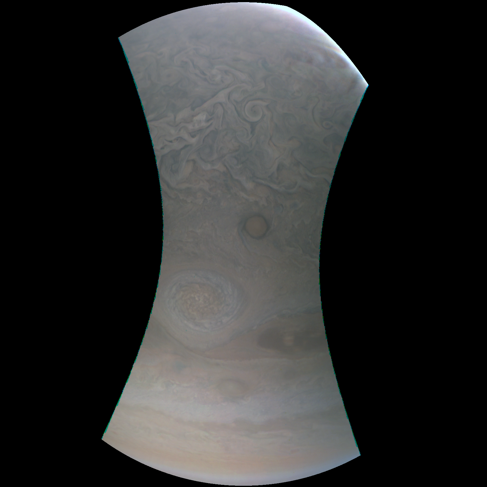
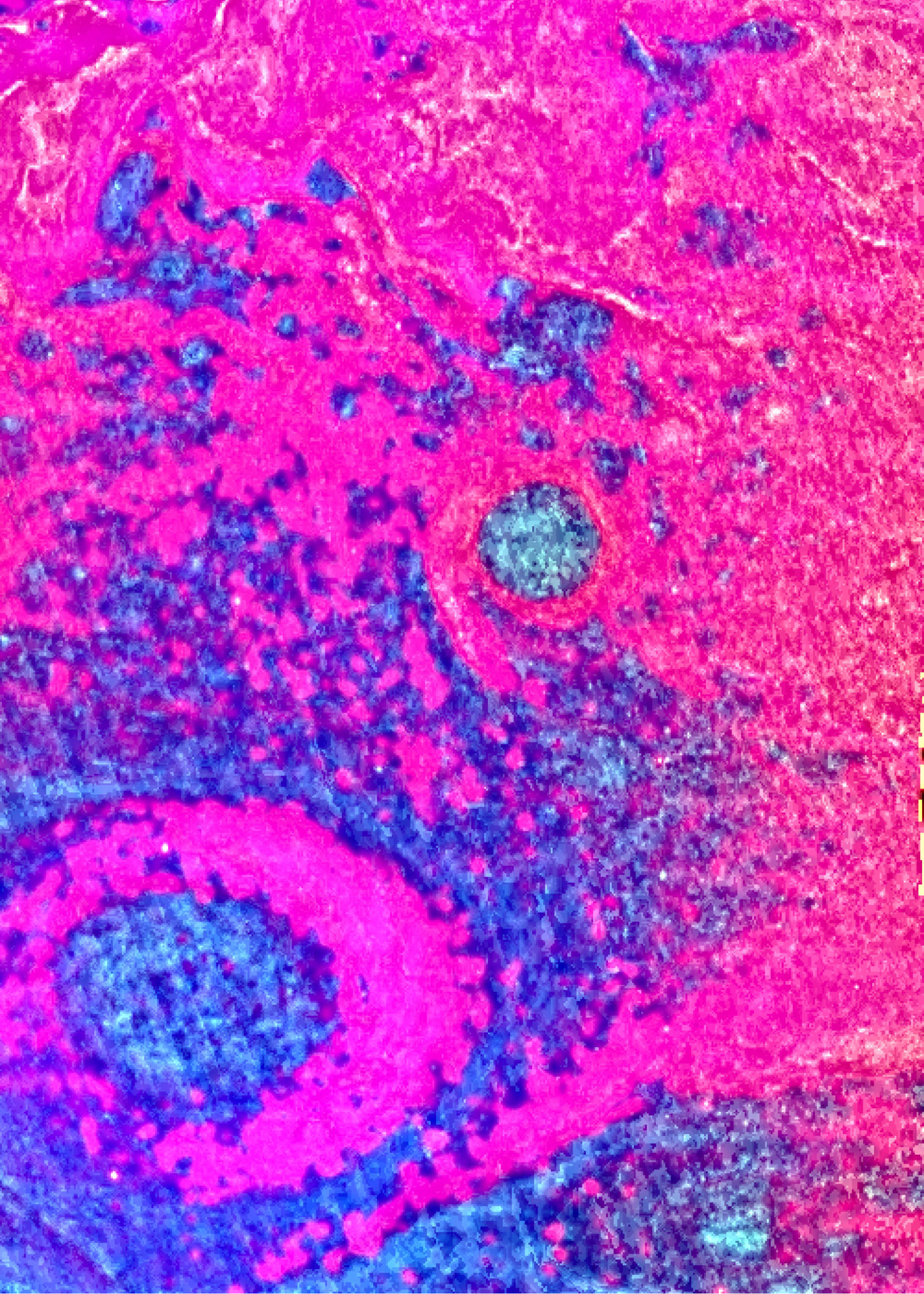
For set 7, I centered the rendering around the dark storm eye and pushed the surrounding atmosphere toward a hurricane-like palette. Smoothing selected structure before remapping the colors makes the composition feel more layered, which helps the central feature read more clearly.

p = ImageCrop[p, {500, 700}];
{hh, ss, bb} = ColorSeparate[p, "HSB"];

bb = GaussianFilter[bb, 5];
hh = GaussianFilter[hh, 5];

out = ColorCombine[{hh * 4, ss * 5, bb * 2}, "RGB"];
out = ImageAdjust[ImageEffect[out, {"DetailEnhancing"}]];

Set 8

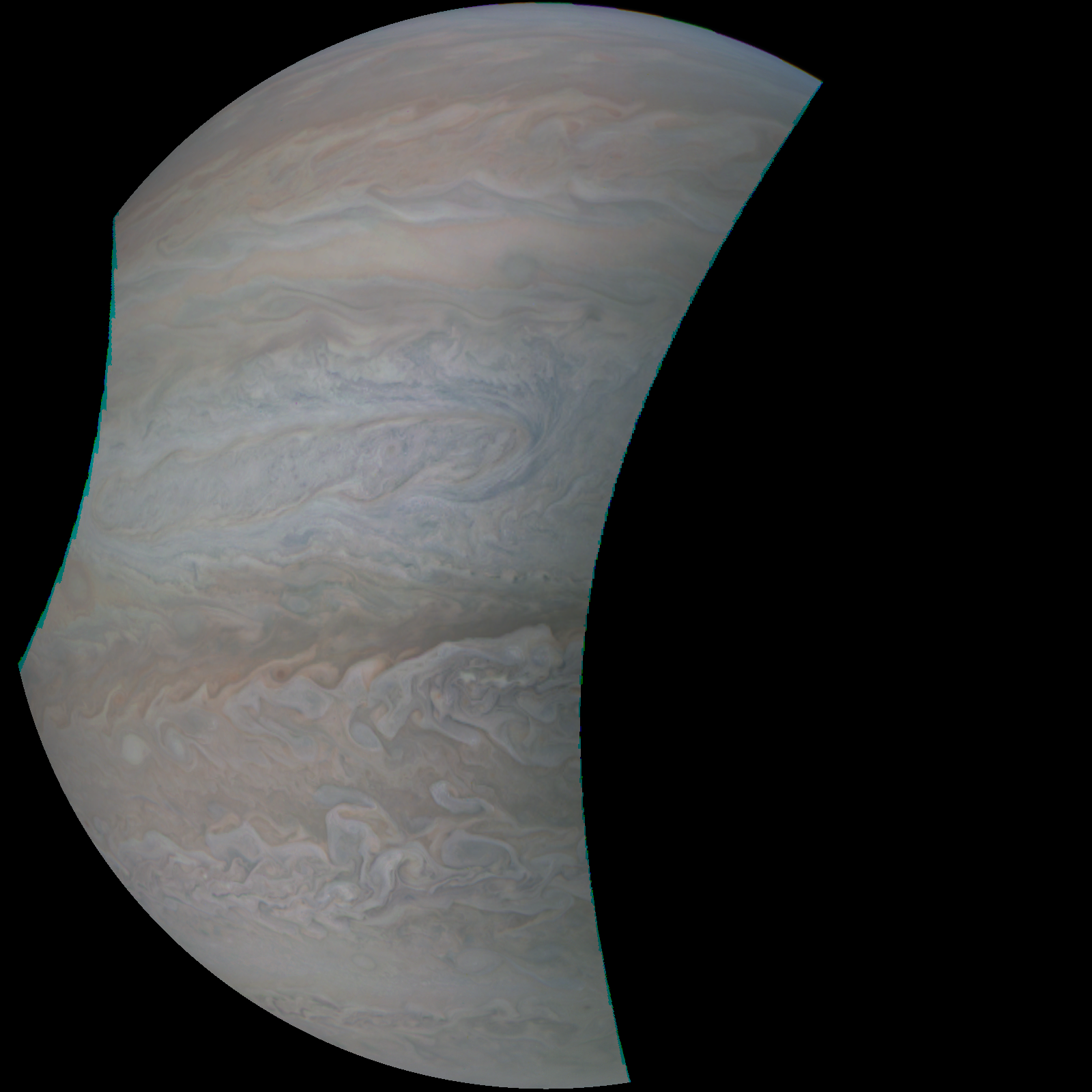
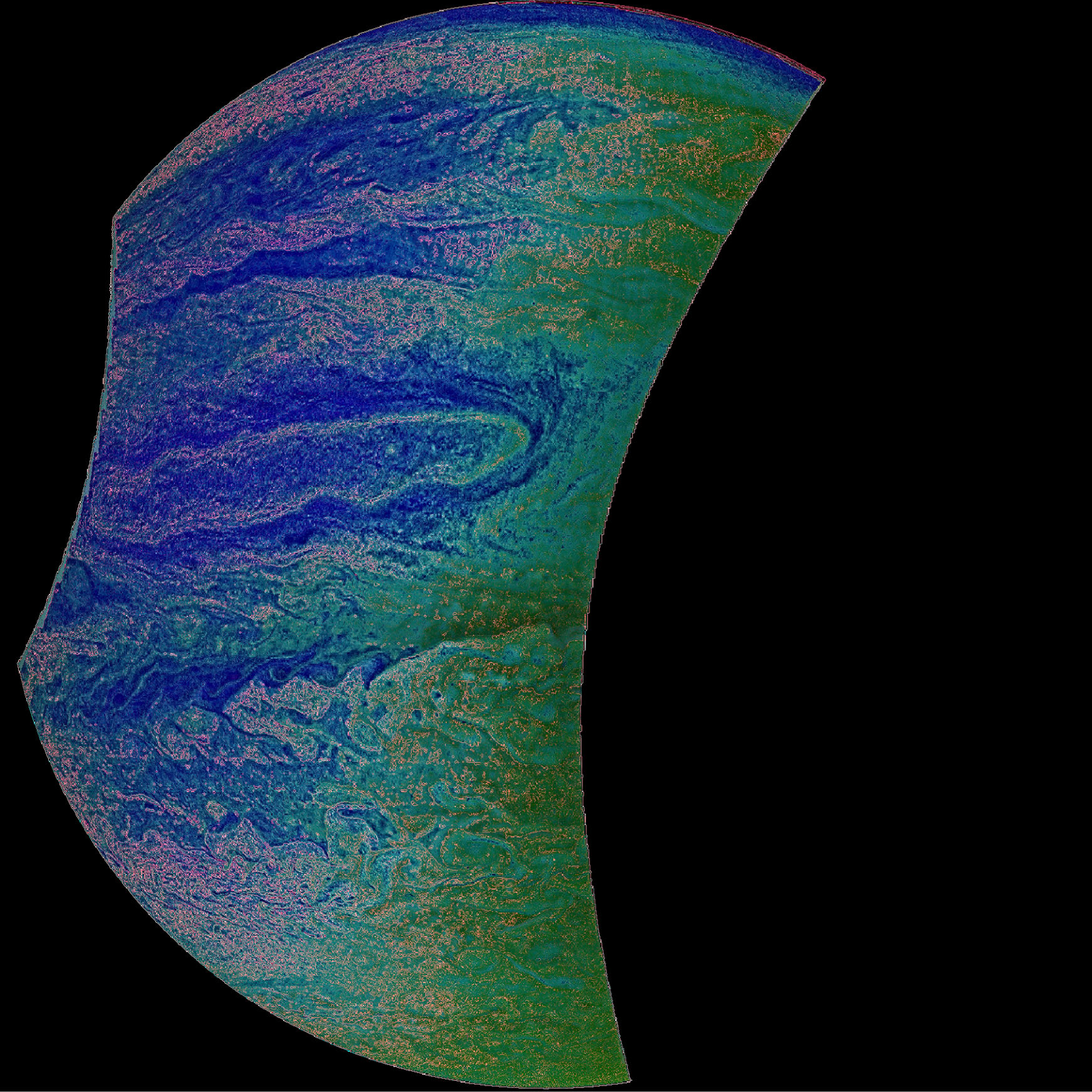
Set 8 focuses on turbulence. Instead of preserving the original channel roles, I remapped them to build a cooler blue-green view that makes the atmosphere feel more active and layered. The enhancement is stylized, but it is driven by the goal of making small-scale structure more legible.

{r, g, b} = ColorSeparate[p, "RGB"];
{hh, ss, bb} = ColorSeparate[p, "HSB"];

out = ColorCombine[{ss + b, hh + r, bb}, "HSB"];
edgeimg = ColorCombine[
  {LaplacianFilter[hh, 1], LaplacianFilter[bb, 1], LaplacianFilter[bb, 1]},
  "RGB"
];

out = ImageCompose[edgeimg, {out, 0.9}];
out = ImageAdd[out, edgeimg];
out = ImageAdjust[ImageEffect[out, {"DetailEnhancing"}]];

Set 9

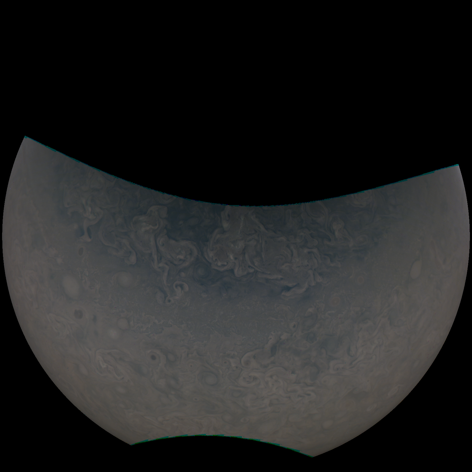
For set 9, I wanted the swirling structure to dominate the image. The enhancement repeatedly strengthens local contrast and then turns that structure into the driver for the final color rendering. That pushes the result further away from literal appearance, but it makes the flow of the atmosphere much easier to see.

out = ImageAdjust[p];
newp = ImageEffect[p, {"DetailEnhancing"}];
out = ImageCompose[out, {newp, 0.8}];
out = ImageEffect[out, {"DetailEnhancing"}];

gray = ColorConvert[out, "Grayscale"];
out = ColorCombine[{g, r, gray}, "HSB"];
out = ImageCompose[gray, {out, 0.8}];
out = ImageEffect[out, {"DetailEnhancing"}];

What I learned

This project made reverse engineering feel much more concrete to me. For the first three sets, channelwise numerical fitting turned out to be an effective way to approximate an existing enhancement pipeline. At the same time, that only works because of a strong assumption: the original enhancement has to behave mostly like a separate weighted remapping of each channel. When that assumption is reasonably true, the reconstruction gets surprisingly close. When it is not, the gap between the target and the prediction becomes obvious, and even extra cleanup still does not fully recover the reference image.

The later sets were a different kind of lesson. For image sets 4 through 9, I had fun applying a range of operations I learned throughout the course and seeing how much structure could be revealed by changing color roles, local contrast, texture, or edge emphasis. Several of those transformations made atmospheric patterns visible that were not nearly as apparent in the original image. That reminded me of augmentation in computer vision: controlled transformations can expose structure, improve robustness, and make a model less dependent on one narrow presentation of the data. Here I was not training a model, but the idea felt related. A carefully chosen transformation can surface information that is present in the image, yet easy to miss without a different view of it.