Building YOLO From Scratch for Real-Time Object Detection
Paper Context
The background reading centered on why YOLO was such a sharp departure from earlier detection systems. Instead of a multi-stage pipeline that proposes regions and then classifies them, YOLO turns detection into a single regression problem over a grid, predicting box coordinates, confidence values, and class probabilities in one forward pass.
That shift from proposal-based detection to direct regression is what drove most of the implementation work. The difficult parts were target encoding, loss bookkeeping, and the post-processing needed to turn dense grid predictions back into final boxes.
Implementation Walkthrough
The sections below cover target generation, network design, loss computation, and a few representative detections from the trained model.
What is the Object Detection?
In image classification, the entire image is classified with a single label.
In object detection, the network localizes one or more objects and predicts a class for each one.
The output is therefore a list of bounding boxes, class labels, and probability/confidence scores.
About YOLO (Main idea)
YOLO is an algorithm for object detection
They reframe object detection as a , straight from image pixels to bounding box coordinates and class probabilities
Using YOLO, you only look once (YOLO) at an image to predict what objects are present and where they are
The main appeal of YOLO is speed: by treating detection as a single regression problem, it avoids the heavier multi-stage pipeline used by earlier detectors.
The main architectural difference from earlier detectors is that localization and classification are predicted together in one forward pass rather than in separate proposal and refinement stages.
Building a YOLO with PyTorch
YOLO model:
22Convolutional Layers
Note that, first and 20th conv layers have stride 2 for halving output size
4 Max Pooling Layers
2 Fully Connected Layers
Leaky ReLu Activation for all layers except for the last layer
Implementing YOLO
The input image is divided into an S S grid of cells
Each grid cell predicts B (=2) bounding boxes as well as C (=20) class probabilities
Each bounding box consists of 5 predictions: x, y, w, h, and confidence
The (x,y) coordinates represent the center of the box relative to the bounds of the grid cell
The width and height are predicted relative to the whole image
If no object exists in that cell, the confidence score is zero.
If the cell contains objects, the confidence score is equal to the intersection over union (IOU) between the predicted box and the ground truth (This is important for building the loss function)
Thus, the output vector is a S S (B 5 + C) (= 7 7 30)
The
generate_targetfunction is central because it constructs the training targets for the grid-based detector output.Load the dataset
Build the YOLO network
The network below follows a simplified YOLO-style detector design.
This implementation follows a simplified variant rather than reproducing the original paper architecture layer-for-layer.
The main implementation work is concentrated in the
self.pre_train_netandself.post_netblocks.All layers use Leaky ReLU with a 0.01 negative slope in this implementation variant.
self.pre_train_net
Name Filters Output Dimension Padding Conv 1 7 x 7 x 64, stride=2 224 x 224 x 64 3 LeakyReLU negative_slop=0.01 224 x 224 x 64 Max Pool 1 2 x 2, stride=2 112 x 112 x 64 Conv 2 3 x 3 x 192 112 x 112 x 192 1 LeakyReLU negative_slop=0.01 112 x 112 x 192 Max Pool 2 2 x 2, stride=2 56 x 56 x 192 Conv 3 1 x 1 x 128 56 x 56 x 128 0 LeakyReLU negative_slop=0.01 56 x 56 x 128 Conv 4 3 x 3 x 256 56 x 56 x 256 1 LeakyReLU negative_slop=0.01 56 x 56 x 256 Conv 5 1 x 1 x 256 56 x 56 x 256 0 LeakyReLU negative_slop=0.01 56 x 56 x 256 Conv 6 3 x 3 x 512 56 x 56 x 512 1 LeakyReLU negative_slop=0.01 56 x 56 x 512 Max Pool 3 2 x 2, stride=2 28 x 28 x 512 Conv 7 1 x 1 x 256 28 x 28 x 256 0 LeakyReLU negative_slop=0.01 28 x 28 x 256 Conv 8 3 x 3 x 512 28 x 28 x 512 1 LeakyReLU negative_slop=0.01 28 x 28 x 512 Conv 9 1 x 1 x 256 28 x 28 x 256 0 LeakyReLU negative_slop=0.01 28 x 28 x 256 Conv 10 3 x 3 x 512 28 x 28 x 512 1 LeakyReLU negative_slop=0.01 28 x 28 x 512 Conv 11 1 x 1 x 256 28 x 28 x 256 0 LeakyReLU negative_slop=0.01 28 x 28 x 256 Conv 12 3 x 3 x 512 28 x 28 x 512 1 LeakyReLU negative_slop=0.01 28 x 28 x 512 Conv 13 1 x 1 x 256 28 x 28 x 256 0 LeakyReLU negative_slop=0.01 28 x 28 x 256 Conv 14 3 x 3 x 512 28 x 28 x 512 1 LeakyReLU negative_slop=0.01 28 x 28 x 512 Conv 15 1 x 1 x 512 28 x 28 x 512 0 LeakyReLU negative_slop=0.01 28 x 28 x 512 Conv 16 3 x 3 x 1024 28 x 28 x 1024 1 LeakyReLU negative_slop=0.01 28 x 28 x 1024 Max Pool 4 2 x 2, stride=2 14 x 14 x 1024 Conv 17 1 x 1 x 512 14 x 14 x 512 0 LeakyReLU negative_slop=0.01 14 x 14 x 512 Conv 18 3 x 3 x 1024 14 x 14 x 1024 1 LeakyReLU negative_slop=0.01 14 x 14 x 1024 self.post_net
Name Filters Output Dimension Padding Conv 19 3 x 3 x 1024 14 x 14 x 1024 1 LeakyReLU negative_slop=0.01 14 x 14 x 1024 Conv 20 3 x 3 x 1024, stride=2 7 x 7 x 1024 1 LeakyReLU negative_slop=0.01 7 x 7 x 1024 Conv 21 3 x 3 x 1024 7 x 7 x 1024 1 LeakyReLU negative_slop=0.01 7 x 7 x 1024 Conv 22 3 x 3 x 1024 7 x 7 x 1024 1 LeakyReLU negative_slop=0.01 7 x 7 x 1024 Loss function
The loss implementation combines localization, confidence, and classification terms in the standard YOLO style.
The full objective is split into localization, confidence, and classification terms.
is defined as follows:
1, if an object is present in grid cell and the th bounding box predictor
0, otherwise
YOLO predicts multiple bounding boxes per grid cell (in our case, 2 bounding boxes are predicted)
In train stage, YOLO requires one bounding box predictor to be responsible for each object
The code assigns one predictor to be “responsible” for predicting an object where the predictor has the highest IOU with the ground truth
The loss function is divided into the three sub-sections
Classification ( classes )
Similar to sum-squared error for classification except for term
Note that, we do not penalize classification error when no object is present on the cell (by term)
No object appears in cell
Compute the loss associated with the confidence score for each bounding box predictor
is equal to one when there is no object in the cell, and 0 other wise
Bounding box coordinates (x,y,h,w) regression (4 scalars), and Object confidence
Compute the loss realted to the predicted bounding box position and width/height
Note that width/height are adapted square root before computing the loss
In order to solve the problem that small deviations in large boxes matter less than in small boxes
Compute the loss associated with the confidence score for the cell which is responsible for the object
Following the paper, and
Train Model
With the model and loss defined, the next step is to assemble the training loop.
In practice, using pretrained weights makes the full experiment much more manageable because training the detector from scratch is expensive.
Inference
- The final stage is inference and evaluation.
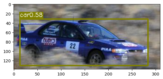
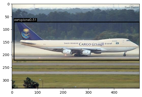
- Qualitative results come from visualizing the predicted boxes and class scores.
- Quantitative evaluation is reported with mean Average Precision (mAP).
Load the dataset
# os.environ["CUDA_VISIBLE_DEVICES"] = "0"

class YoloDataset(data.Dataset):
    def __init__(self, root, list_file, train, transform=None):
        self.image_size = 448
        self.root = root
        self.train = train
        self.transform = transform
        self.fnames = []
        self.boxes = []
        self.labels = []
        self.color_jitter = Compose([transforms.ColorJitter(brightness=0.1,contrast=0.1, saturation=0.1, hue=0.1),
                                                 transforms.ToTensor()])
        self.plain = Compose([transforms.ToTensor()])
        self.resize = Compose([transforms.ToPILImage(),
                              transforms.Resize((self.image_size, self.image_size)),
                              transforms.ToTensor()])

        with open(list_file) as f:
            lines = f.readlines()

        for line in lines:
            splited = line.strip().split()
            self.fnames.append(splited[0])
            num_boxes = (len(splited) - 1) // 5
            box = []
            label = []
            for i in range(num_boxes):
                x_min = float(splited[1+5*i])
                y_min = float(splited[2+5*i])
                x_max = float(splited[3+5*i])
                y_max = float(splited[4+5*i])
                c = splited[5+5*i]
                box.append([x_min, y_min, x_max, y_max])
                label.append(int(c)+1)
            self.boxes.append(torch.Tensor(box))
            self.labels.append(torch.LongTensor(label))
        self.num_samples = len(self.boxes)

    def img_pre_process(self, img, boxes, labels):

        if random.random() < 0.5:
            im_lr = np.fliplr(img).copy()
            height, width, c = img.shape
            x_min = width - boxes[:, 2]
            x_max = width - boxes[:, 0]
            boxes[:,0] = x_min
            boxes[:,2] = x_max
            img = im_lr

        ## Converting the image and box information scaling
        if random.random() < 0.5:
            scale = random.uniform(0.8, 1.2)
            height, width, c = img.shape
            img = cv2.resize(img, (int(width * scale), height))
            boxes = boxes * torch.FloatTensor([[scale, 1, scale, 1]]).expand_as(boxes)

        ## Image translation
        if random.random() < 0.5:
            center = (boxes[:,2:] + boxes[:,:2]) / 2
            height, width, c = img.shape
            shifted_img = np.zeros((height, width, c), dtype=img.dtype)

            w_range = int(random.uniform(-width*0.2, width*0.2))
            h_range = int(random.uniform(-height*0.2, height*0.2))

            if w_range<0 and h_range<0:
                shifted_img[:height+h_range,:width+w_range,:] = img[-h_range:,-w_range:,:]

            elif w_range<0 and h_range>=0:
                shifted_img[h_range:,:width+w_range,:] = img[:height-h_range,-w_range:,:]

            elif w_range>=0 and h_range>=0:
                shifted_img[h_range:,w_range:,:] = img[:height-h_range,:width-w_range,:]

            elif w_range>=0 and h_range<0:
                shifted_img[:height+h_range,w_range:,:] = img[-h_range:,:width-w_range,:]

            wh_range = torch.FloatTensor([[w_range, h_range]]).expand_as(center)
            center = center + wh_range

            mask1 = (center[:,0] > 0) & (center[:,0] < width)
            mask2 = (center[:,1] > 0) & (center[:,1] < height)
            mask = (mask1 & mask2).view(-1,1).bool()

            boxes_in = boxes[mask.expand_as(boxes)].view(-1,4)

            if len(boxes_in) != 0:
                box_shift = torch.FloatTensor([[w_range, h_range, w_range, h_range]]).expand_as(boxes_in)
                boxes_in = boxes_in + box_shift

                labels_in = labels[mask.view(-1)]
                labels = labels_in
                img = shifted_img
                boxes = boxes_in

        ## Image cropping
        if random.random() < 0.5:
            center = (boxes[:,2:] + boxes[:,:2]) / 2
            height, width, c = img.shape
            h = int(random.uniform(0.6*height,height))
            w = int(random.uniform(0.6*width,width))
            x = int(random.uniform(0,width-w))
            y = int(random.uniform(0,height-h))

            center = center - torch.FloatTensor([[x, y]]).expand_as(center)
            mask1 = (center[:,0]>0) & (center[:,0]<w)
            mask2 = (center[:,1]>0) & (center[:,1]<h)
            mask = (mask1 & mask2).view(-1, 1).bool()

            boxes_in = boxes[mask.expand_as(boxes)].view(-1,4)

            if (len(boxes_in)!=0):
                box_shift = torch.FloatTensor([x,y,x,y]).expand_as(boxes_in)

                boxes_in = boxes_in - box_shift
                boxes_in[:,0]=boxes_in[:,0].clamp_(min=0,max=w)
                boxes_in[:,2]=boxes_in[:,2].clamp_(min=0,max=w)
                boxes_in[:,1]=boxes_in[:,1].clamp_(min=0,max=h)
                boxes_in[:,3]=boxes_in[:,3].clamp_(min=0,max=h)

                labels = labels[mask.view(-1)]
                img_cropped = img[y:y+h, x:x+w, :]
                boxes = boxes_in
                img = img_cropped

        return img, boxes, labels

    def generate_target(self, img, boxes, labels):
        grid_size = 7
        h,w,_ = img.shape
        boxes /= torch.Tensor([w,h,w,h]).expand_as(boxes) # Converting the box size 0 ~ 1
        target = torch.zeros((grid_size, grid_size, 30))
        cell_size = 1./grid_size

        wh = boxes[:,2:] - boxes[:,:2]
        cxcy = (boxes[:,2:] + boxes[:,:2]) / 2

        for i in range(cxcy.size()[0]):
            cxcy_sample = cxcy[i] # center pixel
            ij = (cxcy_sample/cell_size).ceil()-1
            target[int(ij[1]),int(ij[0]),4] = 1
            target[int(ij[1]),int(ij[0]),9] = 1
            target[int(ij[1]),int(ij[0]),int(labels[i])+9] = 1

            xy = ij*cell_size
            delta_xy = (cxcy_sample -xy)/cell_size # Converting delta_xy to the size
                                                   # relative to the bounds of the grid cell
            target[int(ij[1]),int(ij[0]),2:4] = wh[i]
            target[int(ij[1]),int(ij[0]),:2] = delta_xy
            target[int(ij[1]),int(ij[0]),7:9] = wh[i]
            target[int(ij[1]),int(ij[0]),5:7] = delta_xy

        return target

    def RandomBrightness(self,bgr):
        if random.random() < 0.5:
            hsv = cv2.cvtColor(bgr,cv2.COLOR_BGR2HSV)
            h,s,v = cv2.split(hsv)
            adjust = random.choice([0.5,1.5])
            v = v*adjust
            v = np.clip(v, 0, 255).astype(hsv.dtype)
            hsv = cv2.merge((h,s,v))
            bgr = cv2.cvtColor(hsv,cv2.COLOR_HSV2BGR)
        return bgr
    def RandomSaturation(self,bgr):
        if random.random() < 0.5:
            hsv = cv2.cvtColor(bgr,cv2.COLOR_BGR2HSV)
            h,s,v = cv2.split(hsv)
            adjust = random.choice([0.5,1.5])
            s = s*adjust
            s = np.clip(s, 0, 255).astype(hsv.dtype)
            hsv = cv2.merge((h,s,v))
            bgr = cv2.cvtColor(hsv,cv2.COLOR_HSV2BGR)
        return bgr
    def RandomHue(self,bgr):
        if random.random() < 0.5:
            hsv = cv2.cvtColor(bgr,cv2.COLOR_BGR2HSV)
            h,s,v = cv2.split(hsv)
            adjust = random.choice([0.5,1.5])
            h = h*adjust
            h = np.clip(h, 0, 255).astype(hsv.dtype)
            hsv = cv2.merge((h,s,v))
            bgr = cv2.cvtColor(hsv,cv2.COLOR_HSV2BGR)
        return bgr

    def randomBlur(self,bgr):
        if random.random()<0.5:
            bgr = cv2.blur(bgr,(5,5))
        return bgr

    def __getitem__(self, idx):
        fname = self.fnames[idx]
        img = cv2.imread(os.path.join(self.root+fname))
        boxes = self.boxes[idx].clone()
        labels = self.labels[idx].clone()

        if self.train:
            img = self.randomBlur(img)
            img = self.RandomBrightness(img)
            img = self.RandomHue(img)
            img = self.RandomSaturation(img)
            img, boxes, labels = self.img_pre_process(img, boxes, labels)

        target = self.generate_target(img, boxes, labels) # 7x7x30

        # Image processing
        img = cv2.cvtColor(img, cv2.COLOR_BGR2RGB)

        img = self.plain(img)
        img = self.resize(img)
        img = 2 * img - 1

        return img, target

    def __len__(self):
        return self.num_samples
Build the YOLO network
The model is defined with
nn.Sequentialbecause the pretrained weights expect that module structure.
class YOLO(nn.Module):
    def __init__(self):
        super(YOLO, self).__init__()

        self.pre_train_net = nn.Sequential(
            ### Fill out ###
            # input = # 448x448x3
            # block 1
            nn.Conv2d(3, 64, 7, stride=2, padding=3),
            nn.LeakyReLU(negative_slope=0.01, inplace=True),
            nn.MaxPool2d(2, stride=2),  # 112x112x64
            # block 2
            nn.Conv2d(64, 192, 3, padding=1),
            nn.LeakyReLU(negative_slope=0.01, inplace=True),
            nn.MaxPool2d(2, stride=2),  # 56x56x192
            # block 3
            nn.Conv2d(192, 128, 1, padding=0),
            nn.LeakyReLU(negative_slope=0.01, inplace=True),
            nn.Conv2d(128, 256, 3, padding=1),
            nn.LeakyReLU(negative_slope=0.01, inplace=True),
            nn.Conv2d(256, 256, 1, padding=0),
            nn.LeakyReLU(negative_slope=0.01, inplace=True),
            nn.Conv2d(256, 512, 3, padding=1),
            nn.LeakyReLU(negative_slope=0.01, inplace=True),
            nn.MaxPool2d(2, stride=2),  # 28x28x512
            # block 4
            nn.Conv2d(512, 256, 1, padding=0),  # conv7
            nn.LeakyReLU(negative_slope=0.01, inplace=True),
            nn.Conv2d(256, 512, 3, padding=1),  # conv8
            nn.LeakyReLU(negative_slope=0.01, inplace=True),
            nn.Conv2d(512, 256, 1, padding=0),  # conv9
            nn.LeakyReLU(negative_slope=0.01, inplace=True),
            nn.Conv2d(256, 512, 3, padding=1),  # conv10
            nn.LeakyReLU(negative_slope=0.01, inplace=True),
            nn.Conv2d(512, 256, 1, padding=0),  # conv11
            nn.LeakyReLU(negative_slope=0.01, inplace=True),
            nn.Conv2d(256, 512, 3, padding=1),  # conv12
            nn.LeakyReLU(negative_slope=0.01, inplace=True),
            nn.Conv2d(512, 256, 1, padding=0),  # conv13
            nn.LeakyReLU(negative_slope=0.01, inplace=True),
            nn.Conv2d(256, 512, 3, padding=1),  # conv14
            nn.LeakyReLU(negative_slope=0.01, inplace=True),
            nn.Conv2d(512, 512, 1, padding=0),  # conv15
            nn.LeakyReLU(negative_slope=0.01, inplace=True),
            nn.Conv2d(512, 1024, 3, padding=1),  # conv16
            nn.LeakyReLU(negative_slope=0.01, inplace=True),
            nn.MaxPool2d(2, stride=2),  # 14x14x1024
            # block 5
            nn.Conv2d(1024, 512, 1, padding=0),
            nn.LeakyReLU(negative_slope=0.01, inplace=True),
            nn.Conv2d(512, 1024, 3, padding=1),
            nn.LeakyReLU(negative_slope=0.01, inplace=True),  # 14x14x1024
        )

        self.post_net = nn.Sequential(
            ### Fill out ###
            nn.Conv2d(1024, 1024, 3, padding=1),  # conv19
            nn.LeakyReLU(negative_slope=0.01, inplace=True),
            nn.Conv2d(1024, 1024, 3, stride=2, padding=1),  # conv20
            nn.LeakyReLU(negative_slope=0.01, inplace=True),
            nn.Conv2d(1024, 1024, 3, padding=1),  # conv21
            nn.LeakyReLU(negative_slope=0.01, inplace=True),
            nn.Conv2d(1024, 1024, 3, padding=1),  # conv22
            nn.LeakyReLU(negative_slope=0.01, inplace=True),  # 7x7x1024
        )

        self.FC1 = nn.Sequential(
            nn.Linear(50176, 4096),
            nn.LeakyReLU(),
            nn.Dropout()
        )

        self.FC2 = nn.Sequential(
            nn.Linear(4096, 1470)
        )

        self.pre_train_net.cuda()
        self.post_net.cuda()
        self.FC1.cuda()
        self.FC2.cuda()

        self._initialize_weights()

    def forward(self, x):
        output = self.pre_train_net(x)
        output = self.post_net(output)

        # Ready to going for FC layer
        output = output.view(output.size(0), -1)

        output = self.FC1(output)
        output = self.FC2(output)

        output = output.view(output.size(0), 7, 7, 30)
        # Converting the output shape to the (batch_size, 7, 7, 30)
        output = F.relu(output)

        return output

    def _initialize_weights(self):
        for m in self.modules():
            if isinstance(m, nn.Conv2d):
                n = m.kernel_size[0] * m.kernel_size[1] * m.out_channels
                m.weight.data.normal_(0, math.sqrt(2. / n))
                if m.bias is not None:
                    m.bias.data.zero_()
            elif isinstance(m, nn.BatchNorm2d):
                m.weight.data.fill_(1)
                m.bias.data.zero_()
            elif isinstance(m, nn.Linear):
                m.weight.data.normal_(0, 0.01)
                m.bias.data.zero_()
Loss function
class yoloLoss(nn.Module):
    def __init__(self,l_coord,l_noobj):
        super(yoloLoss,self).__init__()
        self.l_coord = l_coord
        self.l_noobj = l_noobj

    def compute_prob_error(self, pred, target): ## classification error
        contain = target[:,:,:,4] > 0 # [Batch_size, 7, 7, 1]
        contain = contain.unsqueeze(3).expand_as(target) # [Batch_size, 7, 7, 30]

        ### Fill out ###
        prob_pred = pred[contain].contiguous().view(-1, 30)
        prob_target = target[contain].contiguous().view(-1, 30)
        prob_loss = F.mse_loss(
            prob_pred[:, 10:], prob_target[:, 10:], size_average=False)

        return prob_loss

    def not_contain_obj_error(self, pred, target): ## Error where no object appears in cell
        not_contain = target[:,:,:,4] == 0 # [Batch_size, 7, 7, 1]
        not_contain = not_contain.unsqueeze(3).expand_as(target) # [Batch_size, 7, 7, 30]

        ### Fill out ###
        noobj_pred = pred[not_contain].contiguous().view(-1, 30)
        noobj_target = target[not_contain].contiguous().view(-1, 30)
        noobj_loss1 = F.mse_loss(
            noobj_pred[:, 4:5], noobj_target[:, 4:5], size_average=False)

        return noobj_loss1

    def contain_obj_error(self, pred, target): ##
        contain = target[:,:,:,4] > 0 # [Batch_size, 7, 7, 1]
        contain = contain.unsqueeze(3).expand_as(target) # [Batch_size, 7, 7, 30]

        contain_pred = pred[contain].contiguous().view(-1,30) # Only cell which contains the object are remained
        box_pred = contain_pred[:,:10].contiguous().view(-1,5) # Reshaping

        contain_target = target[contain].contiguous().view(-1,30)
        box_target = contain_target[:,:10].contiguous().view(-1,5)

        # Note that, We assign one predictor to be "responsible" for predicting
        # an object based on which prediction has the highest current IOU with the ground truth
        # Then, other prediction is "not responsible" for predicting an object
        # That component is included in "contain_noobj_mask variables

        contain_obj_mask = torch.cuda.ByteTensor(box_target.size()).zero_().bool() # Create the mask
        contain_noobj_mask = torch.cuda.ByteTensor(box_target.size()).zero_().bool()

        target_iou_gt = torch.zeros(box_target[:,0].size()).cuda() # In order to save the IoU for confidence
                                                                   # of the cell which contains object

        for i in range(0, box_target.size()[0], 2):
            box_p = box_pred[i:i+2] # For 2 bounding boxes information
            box_p_coord = Variable(torch.FloatTensor(box_p.size()))
            box_p_coord[:, :2] = box_p[:, :2]  # Fill out
            box_p_coord[:, 2:4] = box_p[:, 2:4] + box_p[:, :2]  # Fill out

            box_t = box_target[i].contiguous().view(-1, 5)
            box_t_coord = Variable(torch.FloatTensor(box_t.size()))
            box_t_coord[:, :2] = box_t[:, :2]  # Fill out
            box_t_coord[:, 2:4] = box_t[:, 2:4] + box_t[:, :2]  # Fill out

            iou = self.compute_iou(box_p_coord[:,:4], box_t_coord[:,:4]) # [2,]
                                                      # compute IoU between prediction and target boxes,

            gt_iou, max_idx = iou.max(0)
            contain_obj_mask[i+max_idx] = 1
            contain_noobj_mask[i+1-max_idx] = 1

            target_iou_gt[i+max_idx] = gt_iou.data.cuda()

        device = torch.device("cuda" if torch.cuda.is_available() else "cpu")
        target_iou_gt = target_iou_gt.to(device)

        # For the cell which contains object
        contain_box_pred = box_pred[contain_obj_mask].contiguous(
        ).view(-1, 5)  # Fill out

        # For the cell which does not contain object
        not_contain_box_pred = box_pred[contain_noobj_mask].contiguous(
        ).view(-1, 5)  # Fill out

        # For target domain
        contain_box_target = box_target[contain_obj_mask].contiguous(
        ).view(-1, 5)  # Fill out
        not_contain_box_target = box_target[contain_noobj_mask].contiguous(
        ).view(-1, 5)  # Fill out
        not_contain_box_target[:, 4] = 0

        # For the GT IoU
        contain_iou_target = target_iou_gt[contain_obj_mask[:, 4]].contiguous(
        ).view(-1)  # Fill out

        obj_loss = F.mse_loss(contain_box_pred[:,4], contain_iou_target, size_average=False)
        xy_loss = F.mse_loss(contain_box_pred[:,:2], contain_box_target[:,:2], size_average=False)
        wh_loss = F.mse_loss(torch.sqrt(contain_box_pred[:,2:4]), torch.sqrt(contain_box_target[:,2:4]), size_average=False)
        noobj_loss2 = F.mse_loss(not_contain_box_pred[:,4], not_contain_box_target[:,4], size_average=False)

        return obj_loss, xy_loss, wh_loss, noobj_loss2

    def compute_iou(self, box_p, box_t):

        pred_area = (box_p[:,2] - box_p[:,0]) * (box_p[:,3] - box_p[:,1]) # [2,]
        target_area = (box_t[:,2] - box_t[:,0]) * (box_t[:,3] - box_t[:,1]) #[1,]

        box_p = box_p.unsqueeze(1).expand(2,1,4)
        box_t = box_t.unsqueeze(0).expand(2,1,4)

        inter_lt = torch.max(box_p[:,:,:2], box_t[:,:,:2]) # [2,1,2]

        inter_rb = torch.min(box_p[:,:,2:], box_t[:,:,2:]) # [2,1,2]

        wh = inter_rb - inter_lt # [2,1,2]
        wh[wh<0] = 0

        inter_area = wh[:,:,0] * wh[:,:,1] # [2,1]
        pred_area = pred_area.unsqueeze(1).expand_as(inter_area)
        target_area = target_area.unsqueeze(0).expand_as(inter_area)

        iou = inter_area / (pred_area + target_area - inter_area)

        return iou

    def forward(self,pred,target):

        batch_size = pred.size()[0]

        noobj_loss1 = self.not_contain_obj_error(pred, target)
        prob_loss = self.compute_prob_error(pred, target)
        obj_loss, xy_loss, wh_loss, noobj_loss2 = self.contain_obj_error(pred, target)

        total_loss = (self.l_coord*(xy_loss + wh_loss) + obj_loss + self.l_noobj*(noobj_loss1 + noobj_loss2) + prob_loss)

        return total_loss / batch_size
Training the model
import warnings
warnings.filterwarnings("ignore")
file_root = '../dataset-dllab/lab07/all_img/'
train_dataset = YoloDataset(root=file_root, list_file='./misc/lab07/Generate_dataset/voc2007+2012.txt', train=True)
train_loader = DataLoader(train_dataset, batch_size=10, shuffle=True, num_workers=4)

model = YOLO()
state_dict = torch.load('../pretrain/lab07/pre_train.pt')
model.load_state_dict(state_dict['state_dict'])
print('pre_train_complete')

device = torch.device("cuda" if torch.cuda.is_available() else "cpu")
model.to(device)

learning_rate = 1e-4
optimizer = torch.optim.SGD(model.parameters(), lr=learning_rate, momentum=0.9, weight_decay=5e-4)
optimizer.load_state_dict(state_dict['optimizer'])

criterion = yoloLoss(l_coord=5,l_noobj=0.5)

best = 1e+30
num_epochs = 15
print("training start!")

for epoch in range(num_epochs):
    model.train()
    total_loss = 0

    for i, (images, target) in enumerate(train_loader):
        images = images.to(device)
        target = target.to(device)

        pred = model(images)
        loss = criterion(pred, target)

        total_loss += loss.item()

        optimizer.zero_grad()
        loss.backward()
        optimizer.step()

        if (i+1) % 10 == 0:
            print('Epoch [%d/%d], Iter [%d,%d] Loss:%.4f, average_loss: %.4f' % (epoch+1, num_epochs, i+1, len(train_loader), loss.item(), total_loss / (i+1)))
Inference
Inference (Visualizing)
- Below is the visualization code used for the qualitative results.
- The following figures show representative detections from the trained model.
## Visualizing the bouding box image
from misc.lab07.util import *

SMALL_VOC_CLASSES = ('aeroplane', 'bicycle', 'bus', 'car', 'cat', 'dog')

Color = [[0, 0, 0],
                    [128, 0, 0],
                    [0, 128, 0],
                    [128, 128, 0],
                    [0, 0, 128],
                    [128, 0, 128]]

def visualize(model, path):
    result = []
    image = cv2.imread(path)
    h, w, _ = image.shape
    img = cv2.resize(image, (448, 448))
    img = cv2.cvtColor(img, cv2.COLOR_BGR2RGB)

    transform = transforms.Compose([transforms.ToTensor(),])
    img = 2 * transform(img) - 1
    img = Variable(img[None,:,:,:],volatile=True)
    img = img.cuda()

    pred = model(img) #1x7x7x30
    pred = pred.cpu()
    boxes,cls_indexs,probs =  interpret_target(pred, 0.1)

    for i, box in enumerate(boxes):

        x1 = max(int(box[0] * w), 0)
        x2 = min(int(box[2] * w), w)
        y1 = max(int(box[1] * h), 0)
        y2 = min(int(box[3] * h), h)
        cls_index = cls_indexs[i]
        cls_index = int(cls_index)
        prob = probs[i]
        prob = float(prob)
        result.append([(x1, y1), (x2, y2), SMALL_VOC_CLASSES[cls_index], prob])

    img = np.zeros((h, w, 3), np.bool_)
    img = img + image[:,:,::-1]

    for left_up,right_bottom,class_name,prob in result:
        color = Color[SMALL_VOC_CLASSES.index(class_name)]
        cv2.rectangle(img, left_up, right_bottom, color, 2)
        label = class_name+str(round(prob,2))
        text_size, baseline = cv2.getTextSize(label, cv2.FONT_HERSHEY_SIMPLEX, 0.4, 1)
        p1 = (left_up[0], left_up[1]- text_size[1])
        cv2.rectangle(img, (p1[0] - 2//2, p1[1] - 2 - baseline), (p1[0] + text_size[0], p1[1] + text_size[1]), color, -1)
        cv2.putText(img, label, (p1[0], p1[1] + baseline), cv2.FONT_HERSHEY_SIMPLEX, 0.4, (255,255,255), 1, 8)

    print(label)
    plt.imshow(img)

model.eval()
YOLO( (pre_train_net): Sequential( (0): Conv2d(3, 64, kernel_size=(7, 7), stride=(2, 2), padding=(3, 3)) (1): LeakyReLU(negative_slope=0.01, inplace=True) (2): MaxPool2d(kernel_size=2, stride=2, padding=0, dilation=1, ceil_mode=False) (3): Conv2d(64, 192, kernel_size=(3, 3), stride=(1, 1), padding=(1, 1)) (4): LeakyReLU(negative_slope=0.01, inplace=True) (5): MaxPool2d(kernel_size=2, stride=2, padding=0, dilation=1, ceil_mode=False) (6): Conv2d(192, 128, kernel_size=(1, 1), stride=(1, 1)) (7): LeakyReLU(negative_slope=0.01, inplace=True) (8): Conv2d(128, 256, kernel_size=(3, 3), stride=(1, 1), padding=(1, 1)) (9): LeakyReLU(negative_slope=0.01, inplace=True) (10): Conv2d(256, 256, kernel_size=(1, 1), stride=(1, 1)) (11): LeakyReLU(negative_slope=0.01, inplace=True) (12): Conv2d(256, 512, kernel_size=(3, 3), stride=(1, 1), padding=(1, 1)) (13): LeakyReLU(negative_slope=0.01, inplace=True) (14): MaxPool2d(kernel_size=2, stride=2, padding=0, dilation=1, ceil_mode=False) (15): Conv2d(512, 256, kernel_size=(1, 1), stride=(1, 1)) (16): LeakyReLU(negative_slope=0.01, inplace=True) (17): Conv2d(256, 512, kernel_size=(3, 3), stride=(1, 1), padding=(1, 1)) (18): LeakyReLU(negative_slope=0.01, inplace=True) (19): Conv2d(512, 256, kernel_size=(1, 1), stride=(1, 1)) (20): LeakyReLU(negative_slope=0.01, inplace=True) (21): Conv2d(256, 512, kernel_size=(3, 3), stride=(1, 1), padding=(1, 1)) (22): LeakyReLU(negative_slope=0.01, inplace=True) (23): Conv2d(512, 256, kernel_size=(1, 1), stride=(1, 1)) (24): LeakyReLU(negative_slope=0.01, inplace=True) (25): Conv2d(256, 512, kernel_size=(3, 3), stride=(1, 1), padding=(1, 1)) (26): LeakyReLU(negative_slope=0.01, inplace=True) (27): Conv2d(512, 256, kernel_size=(1, 1), stride=(1, 1)) (28): LeakyReLU(negative_slope=0.01, inplace=True) (29): Conv2d(256, 512, kernel_size=(3, 3), stride=(1, 1), padding=(1, 1)) (30): LeakyReLU(negative_slope=0.01, inplace=True) (31): Conv2d(512, 512, kernel_size=(1, 1), stride=(1, 1)) (32): LeakyReLU(negative_slope=0.01, inplace=True) (33): Conv2d(512, 1024, kernel_size=(3, 3), stride=(1, 1), padding=(1, 1)) (34): LeakyReLU(negative_slope=0.01, inplace=True) (35): MaxPool2d(kernel_size=2, stride=2, padding=0, dilation=1, ceil_mode=False) (36): Conv2d(1024, 512, kernel_size=(1, 1), stride=(1, 1)) (37): LeakyReLU(negative_slope=0.01, inplace=True) (38): Conv2d(512, 1024, kernel_size=(3, 3), stride=(1, 1), padding=(1, 1)) (39): LeakyReLU(negative_slope=0.01, inplace=True) ) (post_net): Sequential( (0): Conv2d(1024, 1024, kernel_size=(3, 3), stride=(1, 1), padding=(1, 1)) (1): LeakyReLU(negative_slope=0.01, inplace=True) (2): Conv2d(1024, 1024, kernel_size=(3, 3), stride=(2, 2), padding=(1, 1)) (3): LeakyReLU(negative_slope=0.01, inplace=True) (4): Conv2d(1024, 1024, kernel_size=(3, 3), stride=(1, 1), padding=(1, 1)) (5): LeakyReLU(negative_slope=0.01, inplace=True) (6): Conv2d(1024, 1024, kernel_size=(3, 3), stride=(1, 1), padding=(1, 1)) (7): LeakyReLU(negative_slope=0.01, inplace=True) ) (FC1): Sequential( (0): Linear(in_features=50176, out_features=4096, bias=True) (1): LeakyReLU(negative_slope=0.01) (2): Dropout(p=0.5, inplace=False) ) (FC2): Sequential( (0): Linear(in_features=4096, out_features=1470, bias=True) ) )
- Additional examples can be produced by changing the input image file.
visualize(model, './misc/lab07/Generate_dataset/images/004199.jpg')
visualize(model, './misc/lab07/Generate_dataset/images/006034.jpg')
Inference (mAP)
- Below is the evaluation code used to measure network performance.
- The predicted detections are written to the
Generate_datasetdirectory. - Running
%run ./misc/lab07/Generate_dataset/main.pythen prints the mAP. - In this run, a correct implementation produced an mAP above 69.
import matplotlib.pyplot as plt
%matplotlib inline

SMALL_VOC_CLASSES = ('aeroplane', 'bicycle', 'bus', 'car', 'cat', 'dog')
os.makedirs('predicted', exist_ok=True)

def write(model, path):
    result = []
    image = cv2.imread(path)
    h, w, _ = image.shape
    img = cv2.resize(image, (448, 448))
    img = cv2.cvtColor(img, cv2.COLOR_BGR2RGB)

    transform = transforms.Compose([transforms.ToTensor(),])
    img = 2 * transform(img) - 1
    img = Variable(img[None,:,:,:],volatile=True)
    img = img.cuda()

    pred = model(img) #1x7x7x30
    pred = pred.cpu()
    boxes,cls_indexs,probs =  interpret_target(pred, 0)

    txt_file = open(os.path.join('predicted', os.path.basename(path)[:-4]+'.txt'), 'w')

    for i, box in enumerate(boxes):

        x1 = max(int(box[0] * w), 0)
        x2 = min(int(box[2] * w), w)
        y1 = max(int(box[1] * h), 0)
        y2 = min(int(box[3] * h), h)
        cls_index = cls_indexs[i]
        cls_index = int(cls_index)
        prob = probs[i]
        prob = float(prob)
        txt_file.write(str(SMALL_VOC_CLASSES[cls_index])+' '+'%.6f'%(prob)+' '+str(x1)+' '+str(y1)+' '+str(x2)+' '+str(y2))
        txt_file.write('\n')
    txt_file.close()

import glob

model.eval()
img_names = glob.glob('./misc/lab07/Generate_dataset/images/*')

for i, file_name in enumerate(img_names):
    write(model, file_name)
    if i % 500 == 0:
        print(i)
%run ./misc/lab07/Generate_dataset/main.py
Discussion
The final YOLO run was good enough to clear the expected mAP threshold, with the remaining weaknesses showing up mostly in confidence calibration and small-object behavior.
Quantitative Analysis
The model was trained on PASCAL VOC 2007 and 2012 for 15 epochs with 430 iterations per epoch. Average loss dropped from about 0.58 to 0.48. On the evaluation set, bus was the weakest class, while dog and cat produced the strongest AP scores, both above 70%. The overall mAP cleared 69, which was consistent with the expected range for a correct implementation.
Qualitative Analysis
The example images show that both localization and classification were working, although confidence scores tended to stay in the 50-60% range. The weakness noted in the paper also showed up here: objects that are smaller or farther from the image center are harder for the model, which is one reason finer grids and multi-scale variants became important later on.
References
[1] https://www.pyimagesearch.com/2018/05/14/a-gentle-guide-to-deep-learning-object-detection/