Building Spatial Transformer Networks From Scratch
Paper Context
The background reading framed Spatial Transformer Networks as a response to an implicit weakness in standard CNNs. Pooling and depth can make a classifier somewhat tolerant to translation and deformation, but they do not give the model an explicit mechanism for deciding how an input should be spatially normalized before feature extraction.
STN solves that with a differentiable geometric module: a localization network predicts transformation parameters, a grid generator produces sampling coordinates, and a sampler applies bilinear interpolation so the whole pipeline remains trainable end to end. In practice, the distorted-MNIST run becomes less about raw classifier depth and more about whether the model learns a useful normalization step before recognition.
Implementation Walkthrough
The sections below break down the STN module, the distorted-MNIST setup, and the plain CNN baseline used for comparison.
Spatial Transformer Network for classification of distorted MNIST dataset
Spatial Transformer Network (STN) [1]
- CNNs are limited by the lack of ability to be spatially invariant to the input data
- Learnable module which explicitly allows the spatial manipulation of data within the network
- This differentiable module can be inserted into existing convolutional architectures
STN module
- Localization Network
- With given input feature map, this network outputs the parameters of the spatial transformation (e.g. 6 parameters for affine transformation)
- Reference for affine transformation : [2],[3]
- Parameterised sampling grid (Grid generator)
- Set of points where the input feature map is sampled to produce the transformation which is a output of localization network
- Target coordinate and source coordinate are normalised (, )
- Differentiable Image Sampling (Sampler)
- Ouput feature map is produced by differentiable bilinear interpolation with input feature map and parameterised sampling grid
import warnings
import numpy as np
import torch
import torch.nn as nn
import torch.optim as optim
import torch.nn.init as init
import torchvision.datasets as dset
import torchvision.transforms as transforms
from torch.utils.data import DataLoader
from torch.autograd import Variable
import torch.nn.functional as F
import torchvision.utils as v_utils
import matplotlib.pyplot as plt
from PIL import Image
import cv2
import io
import requests
import os
import copy
import time
%matplotlib inline

warnings.filterwarnings("ignore")
device0 = torch.device("cuda:0" if torch.cuda.is_available() else "cpu")
torch.cuda.get_device_name(0)
‘NVIDIA GeForce RTX 3090’
# parameters

batch_size = 256
learning_rate = 0.001
num_epoch = 60
num_classes = 10
Dataset (Distorted MNIST, details in Appendix A.4 Distorted MNIST)
- Generate RTS(rotated, translated, scaled) MNIST
- Use torchvision.transforms
- Randomly rotating between
- Randomly scaling the digit by a factor of between
- Placing the digit in a random location in a region of image’s center
- Zerp padding to increase image’s size for the digit’s translation ( image)
- Images to tensor
- Normalize data with MNIST dataset’s mean and standard deviation printed in the 5th cell below
Dataset transformation
train_dataset = dset.MNIST(root='../dataset/lab04/MNIST', train=True,
                        transform=transforms.Compose([
                            # Zero padding
                            # (28x28) + pad(26) => (80x80)
                            transforms.Pad(padding=26),
                            # Random rotation, scaling, and translation
                            transforms.RandomAffine(
                                degrees=(-45, 45), scale=(0.7, 1.2), translate=(0.25, 0.25)),
                            transforms.ToTensor(),  # Convert images to tensors
                            transforms.Normalize((0.1307,), (0.3081,)  # Normalize
                                                    )
                        ]),
                        target_transform=None,
                        download=True)
test_dataset = dset.MNIST(root='../dataset/lab04/MNIST', train=False,
                        transform=transforms.Compose([
                            # Zero padding
                            # (28x28) + pad(26) => (80x80)
                            transforms.Pad(padding=26),
                            # Random rotation, scaling, and translation
                            transforms.RandomAffine(
                                degrees=(-45, 45), scale=(0.7, 1.2), translate=(0.25, 0.25)),
                            transforms.ToTensor(),  # Convert images to tensors
                            transforms.Normalize((0.1307,), (0.3081,)  # Normalize
                                                )
                        ]),
                        target_transform=None,
                        download=False)

train_size = len(train_dataset)
test_size = len(test_dataset)

#dataset mean and std for normalization
print('MNIST mean: ',train_dataset.train_data.float().mean()/255)
print('MNIST std: ',train_dataset.train_data.float().std()/255)
print('Train dataset size: {}'.format(len(train_dataset)))
print('Test dataset size: {}'.format(len(test_dataset)))
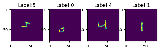
Visualize Dataset
figure = plt.figure()

for i in range(train_size):
    sample = train_dataset[i]
    figure.add_subplot(1,4,i+1).set_title('Label:{}'.format(sample[1]))
    imgplot = plt.imshow((sample[0].squeeze(0).cpu()+1)/2)
    if i == 3:
        plt.show()
        break
train_loader = torch.utils.data.DataLoader(train_dataset,batch_size=batch_size, shuffle=True,num_workers=4,drop_last=True)
test_loader = torch.utils.data.DataLoader(test_dataset,batch_size=batch_size, shuffle=False,num_workers=4,drop_last=True)
Model
CNN Model Setup (details in Appendix A.4 Distorted MNIST)
- CNN
- 2 convolutional layers and 2 max-pooling layers before final classification layer
- Two conv layers have 32 and 64 filters and use ReLU
- Classifier
- 2 fully-connected layers and the number of input features to the last layer is 128
- Also use ReLU as an activation function
- ST module
- At the beginning of the network
- 2 convolutional layer and 2 fully-connected layer in localization network
- Initialize the fc_loc’s final regression layer with identity transformation
- Produce affine transformation parameters for RTS dataset
- Reference for grid generator function: [4]
- Reference for sampler function: [5]
++For RTS datasets, the network has average pooling layer after the ST module to downsample the output of the transformer by a factor of 2
| Layer | Kernel size | stride | padding |
|---|---|---|---|
| 1st Conv of cnn | 9 | 1 | 0 |
| 2nd Conv of cnn | 7 | 1 | 0 |
| 1st Conv of localization | 5 | 1 | 0 |
| 2nd Conv of localization | 5 | 1 | 0 |
| AvgPool | 2 | 2 | 0 |
| MaxPool | 2 | 2 | 0 |
Model class (STN_CNN)
class STN_CNN(nn.Module):

    def __init__(self):
        super(STN_CNN, self).__init__()

        # CNN
        self.cnn = nn.Sequential(
            nn.AvgPool2d(kernel_size=2, stride=2), # Average Pooling after STN
            nn.Conv2d(1, 32, kernel_size=9, stride=1),
            nn.ReLU(inplace=True),
            nn.MaxPool2d(2, stride=2),
            nn.Conv2d(32, 64, kernel_size=7, stride=1),
            nn.ReLU(inplace=True),
            nn.MaxPool2d(2, stride=2)
        )

        # Classifier
        self.classifier = nn.Sequential(
            nn.Linear(1600, 128),  # 1600 = 64 x 5 x 5
            nn.ReLU(inplace=True),
            nn.Linear(128, 10),
            nn.LogSoftmax(dim=1) # use softmax classifier ref [A.4]
        )

        # Localization Network (Convolution)
        self.localization = nn.Sequential(
            nn.Conv2d(1, 20, kernel_size=5, stride=1),
            nn.MaxPool2d(2, stride=2),
            nn.ReLU(inplace=True),
            nn.Conv2d(20, 20, kernel_size=5, stride=1),
            nn.ReLU(inplace=True),
        )

        # Localization Network (Fully Connected)
        self.fc_loc = nn.Sequential(
            nn.Linear(23120, 20),  # 23120 = 20 x 34 x 34
            nn.ReLU(inplace=True),
            nn.Linear(20, 6)
        )

        # Initialize fc_loc weights and biases to Identity (zero weights, identity transform bias)
        self.fc_loc[2].weight.data.zero_()
        self.fc_loc[2].bias.data.copy_(torch.tensor(
            [1, 0, 0, 0, 1, 0], dtype=torch.float))

    def stn(self, x):
        xs = self.localization(x)
        xs = xs.view(-1, 20 * 34 * 34)
        theta = self.fc_loc(xs)
        theta = theta.view(-1, 2, 3)

        grid = F.affine_grid(theta, x.size())  # ref[4]
        x = F.grid_sample(x, grid)  # ref[5]
        return x

    def forward(self, x):
        # Transform the input using STN at the start of the network
        x = self.stn(x)

        # Classification Network
        x = self.cnn(x)
        x = x.view(-1, 64 * 5 * 5)
        x = self.classifier(x)

        return x
model = STN_CNN()

print("STN_CNN's state_dict:")
os.makedirs('weights/lab04', exist_ok=True)
for param_tensor in model.state_dict():
    print(param_tensor, "\t", model.state_dict()[param_tensor].size())
Parameter updates
Scheduling (Annealing) the learning rate [6]
- In training deep networks, it is usually helpful to anneal the learning rate over time
- With high learning rate, the optimizing system can’t settle down into deeper parts of the loss function
- When to decay can be tricky
- Slowly : Wasting computation with little improvement for a long time
- Aggressively: Cooling too quickly, unable to find the best point
- 3 common types
- Step decay: Reduce the learning rate by some factor every few epochs (e.g. half every 5 epochs, or by 0.1 every 10 epochs)
- Exponential decay: In the form of mathematical formulation , where are hyperparameters and is the iteration number(or units of epochs)
- decay : In the form of mathematical formulation , where are hyperparameters and is the iteration number
- In practice, the step decay is slightly preferable
How to adjust learning rate in pytorch [7]
- torch.optim.lr_scheduler provides several methods based on the number of epochs
- For example, the step decay can be implemented by torch.optim.lr_scheduler.StepLR class (See reference for more types)
- This implementation uses ReduceLROnPlateau, which adjusts the learning rate dynamically based on validation measurements
- Reduce the learning rate when our metric has stopped improving
- The learning rate is reduced if no improvement of our metric is seen for a ‘patience’ number of epochs
- See reference for more details
optimizer = torch.optim.Adam(model.parameters(), lr=learning_rate)
scheduler = optim.lr_scheduler.ReduceLROnPlateau(optimizer, mode='max', factor = 0.1, patience=6)

def get_lr(optimizer):
    for param_group in optimizer.param_groups:
        return param_group['lr']
Train/Test
Tirain the STN_CNN model and print accuracy for every epochs
'''
Training options specified in the paper:
optim = SGD #! <- Adam
150k iter
batch_size = 256
base_lr = 0.01 #! <- 0.001
weight_decay = False
dropout = False
lr = lr/10 every50k_iter #! <- ReduceLROnPlateau
'''

# cross entropy loss specified in 4.1 Distorted MNIST
criterion = nn.CrossEntropyLoss()

# Model to GPU
model.to(device0)

best_acc = 0

for epoch in range(num_epoch):
    #TRAIN
    model.train()
    start = time.time()

    for j,(img,label) in enumerate(train_loader):

        # load to gpu
        img = img.to(device0)
        label = label.to(device0)

        # Forward
        outputs = model(img)
        loss = criterion(outputs, label)

        # Backward
        optimizer.zero_grad()  # clear gradients
        loss.backward()  # calculate gradients
        optimizer.step()  # update parameters

        if j % 200 == 0:

            print('Train Epoch: {} [{}/{} ({:.0f}%) / Learning rate:{}]\tLoss:{:.6f}  '.format(
                    epoch, j * len(img), train_size,
                    100. * j / len(train_loader),get_lr(optimizer), loss.item()))

    #Test
    model.eval()
    correct = 0
    total = 0
    for k, (img, label) in enumerate(test_loader):

        # load to gpu
        img = img.to(device0)
        label = label.to(device0)

        # Forward
        outputs = model(img)
        # Get predictions from the maximum value
        _, predicted = torch.max(outputs.data, 1)

        # Total number of labels
        total += label.size(0)

        # Total correct predictions
        if torch.cuda.is_available():  # if pred & label should be in cpu for computation
            correct += (predicted.cpu() == label.cpu()).sum()
        else:
            correct += (predicted == label).sum()

    accuracy = 100 * correct.item() / test_size

    print(f'Test set accuracy: {correct.item()}/{test_size} ({accuracy}%)')

    print('////Epoch elapsed time: {}////\n'.format(time.time() - start))

    if accuracy > best_acc :
        torch.save({
            'epoch': epoch,
            'model_state_dict': model.state_dict(),
            'optimizer_state_dict': optimizer.state_dict(),
            'loss': loss,
            'accuracy': accuracy

            }, './weights/lab04/best_model_STN.tar')

        best_acc = accuracy

    scheduler.step(accuracy)
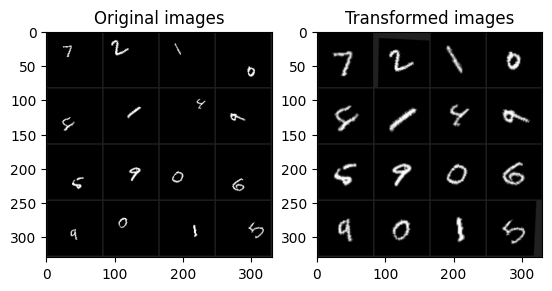
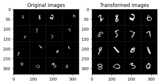
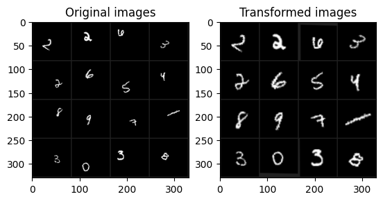
Visualize original inputs and transformed inputs with best pre-trained model
model = STN_CNN()
checkpoint = torch.load('./weights/lab04/best_model_STN.tar')
model.load_state_dict(checkpoint['model_state_dict'])
Our pretrained model’s best accuracy
print('Best accuracy of our model with ST module: ', checkpoint['accuracy'])
# Tensor image to array image
def reprocess_image(img):

    img_re = copy.copy(img.cpu().data.numpy())

    mean = [-0.1307,-0.1307,-0.1307]
    std = [1/0.3081,1/0.3081,1/0.3081]

    for c in range(3):
        img_re[c,:,:] /= std[c]
        img_re[c,:,:] -= mean[c]

    img_re[img_re > 1] = 1
    img_re[img_re < 0] = 0

    img_re = img_re.transpose(1,2,0)

    return img_re
Visualizing original and transformed inputs
- VisualizeSTN class with an input of our pretrained model
- forward_stn: Forward pass of our pretrained STN module to produce transformed inputs
- visualize: Visualizing the original inputs and the transformed ones in a grid
- Forward pass of STN module to produce the transformed inputs
- Unnormalize both images using reprocess_image function
- Make grids of them
- Visualize
class VisualizeSTN():

    def __init__(self, model):
        self.model = model
        self.model.to(device0)
        self.model.eval()

    # Output transformed inputs
    def forward_stn(self,x):
        output = self.model.stn(x)
        return output

    def visualize(self, img):
        # get stn image
        stn_img = self.forward_stn(img)

        # expand channels BW -> RGB
        img = torch.cat((img, img, img), dim=1)
        stn_img = torch.cat((stn_img, stn_img, stn_img), dim=1)

        # make grid of each tensors
        grid_img = v_utils.make_grid(img, nrow=4)
        grid_stn = v_utils.make_grid(stn_img, nrow=4)

        # denormalize and convert to numpy array
        grid_img = reprocess_image(grid_img)
        grid_stn = reprocess_image(grid_stn)

        #

        figure = plt.figure()

        figure.add_subplot(1, 2, 1).set_title(f'Original images')
        imgplot = plt.imshow(grid_img)
        figure.add_subplot(1, 2, 2).set_title(f'Transformed images')
        imgplot = plt.imshow(grid_stn)

        plt.show()

        return
visualize_stn = VisualizeSTN(model)
for i, (image,label) in enumerate(test_loader):

    img = image[:16].to(device0)
    visualize_stn.visualize(img)

    if (i+1) == 3:
        break
Comparison with the cnn model without ST module
- Model composed of cnn and classifier modules same with our pretrained CNN_STN model
- The comparison model reuses the previously defined cnn and classifier modules.
Model class
class CNN(STN_CNN):
    def __init__(self):
        super(CNN, self).__init__()
        self.localization = None
        self.fc_loc = None

    def forward(self, x):
        # Classification Network
        x = self.cnn(x)
        x = x.view(-1, 64 * 5 * 5)
        x = self.classifier(x)

        return x
model_nostn = CNN()

print("CNN's state_dict:")
for param_tensor in model_nostn.state_dict():
    print(param_tensor, "\t", model_nostn.state_dict()[param_tensor].size())
optimizer = torch.optim.Adam(model_nostn.parameters(), lr=learning_rate)
scheduler = optim.lr_scheduler.ReduceLROnPlateau(optimizer, mode='max', factor = 0.1, patience=6)

def get_lr(optimizer):
    for param_group in optimizer.param_groups:
        return param_group['lr']
Train/Test
# cross entropy loss ref [4.1 Distorted MNIST]
criterion = nn.CrossEntropyLoss()

# Model to GPU
model_nostn.to(device0)

best_acc = 0

for epoch in range(num_epoch):
    # TRAIN
    model_nostn.train()
    start = time.time()

    for j, (img, label) in enumerate(train_loader):

        # load to gpu
        img = img.to(device0)
        label = label.to(device0)

        # Forward
        outputs = model_nostn(img)
        loss = criterion(outputs, label)

        # Backward
        optimizer.zero_grad()  # clear gradients
        loss.backward()  # calculate gradients
        optimizer.step()  # update parameters

        if j % 200 == 0:

            print('Train Epoch: {} [{}/{} ({:.0f}%) / Learning rate:{}]\tLoss:{:.6f}  '.format(
                epoch, j * len(img), train_size,
                100. * j / len(train_loader), get_lr(optimizer), loss.item()))

    # Test
    model_nostn.eval()

    correct = 0
    total = 0
    for k, (img, label) in enumerate(test_loader):

        # load to gpu
        img = img.to(device0)
        label = label.to(device0)

        # Forward
        outputs = model_nostn(img)
        # Get predictions from the maximum value
        _, predicted = torch.max(outputs.data, 1)

        # Total number of labels
        total += label.size(0)

        # Total correct predictions
        if torch.cuda.is_available():  # if pred & label should be in cpu for computation
            correct += (predicted.cpu() == label.cpu()).sum()
        else:
            correct += (predicted == label).sum()

    accuracy = 100 * correct.item() / test_size

    print(f'Test set accuracy: {correct.item()}/{test_size} ({accuracy}%)')

    print('////Epoch elapsed time: {}////\n'.format(time.time() - start))

    if accuracy > best_acc:
        torch.save({
            'epoch': epoch,
            'model_state_dict': model_nostn.state_dict(),
            'optimizer_state_dict': optimizer.state_dict(),
            'loss': loss,
            'accuracy': accuracy

        }, './weights/lab04/best_model_noSTN.tar')

        best_acc = accuracy

    scheduler.step(accuracy)
Best accuracy of the model without ST module
print('Best accuracy of our model without ST module: ', best_acc)
References
[1] https://arxiv.org/pdf/1506.02025.pdf
[2] https://en.wikipedia.org/wiki/Affine_transformation
[3] https://en.wikipedia.org/wiki/Transformation_matrix#Affine_transformations
[4] https://pytorch.org/docs/stable/nn.html#affine-grid
[5] https://pytorch.org/docs/stable/nn.html#torch.nn.functional.grid_sample
[6] http://cs231n.github.io/neural-networks-3/#anneal
[7] https://pytorch.org/docs/stable/optim.html#how-to-adjust-learning-rate
Discussion
The main result from this experiment was that the learned transformation made the downstream classifier noticeably more stable.
Qualitative Assessment
The STN visualizations around the later cells show the network learning to center and normalize the distorted digits before classification. Once that transformation is applied, the downstream CNN receives a much more consistent feature pattern than it does from the unaligned inputs.
Quantitative Assessment
The accuracy comparison points in the same direction: the STN-equipped CNN reached 98.94%, compared with 97.38% for the plain CNN, without needing a large increase in parameters or a separate augmentation-heavy pipeline for every distortion pattern.