Building Fully Convolutional Networks From Scratch for Semantic Segmentation
Paper Context
The background reading reframed semantic segmentation as a dense prediction problem rather than a slight extension of classification. Standard CNN classifiers repeatedly pool away spatial detail and then collapse the representation into fully connected layers, which is exactly the opposite of what a pixel-wise labeling task needs.
Fully Convolutional Networks addressed that mismatch by turning a classifier backbone into a dense predictor and then recovering detail with skip connections and learned upsampling. That progression is also how this implementation is organized, starting from convolutionalized VGG features and ending with FCN-style fusion and decoding.
Implementation Walkthrough
The sections below move from convolutionalized VGG features to dense prediction and then to the segmentation outputs from the experiment.
What is Semantic Segmentation?
Semantic segmentation is an approach to understand what is in the image in pixel-level:
-
It is a lot more difficult than image classification, which makes a prediction in image-level.
-
It differs from object detection in that it has no information about instances.
Applications for semantic segmentation include:
-
Autonomous driving
-
Image Editing
-
Classification of terrain visible in satellite imagery
-
Medical imaging analysis
Semantic segmentation with CNNs
-
Typical classification models (AlexNet, VGGNet, …) take fixed-sized inputs and produce a probability vector. The fully connected layers of these models have fixed dimensions and throw away spatial coordinates.
-
It is known that the fully connected layer can be viewed as a convolution layer with a kernel that covers only one pixel, that is, a 1x1 kernel. Thus, we can convert the fully connected layers into convolution layers with maintaining pre-trained weights.
-
After ‘convolutionalizing’ fully connected layers, a feature map needs to be upsampled because of pooling operations in the models. Instead of using simple bilinear interpolation, we can use a transposed convolution layer to learn the interpolation process. This layer is also called as upconvolution, deconvolution or fractionally-strided convolution.
Pixel wise classification using sliding window
This baseline treats segmentation as repeated image classification on overlapping crops, which is both slow and poor at recovering clean object boundaries.
1 Example with VGG-Net
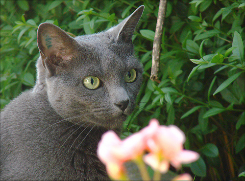
Load a test image
from PIL import Image
test_img_path = '../dataset-dllab/lab06/img/2009_005160.jpg'
test_img = Image.open(test_img_path)
test_img
Standardization of the test image
import torchvision.transforms as transforms
normalize = transforms.Normalize(mean=[0.485, 0.456, 0.406], std=[0.229, 0.224, 0.225])

transform = transforms.Compose([
    transforms.Resize(256),
    transforms.CenterCrop(224),
    transforms.ToTensor(),
    normalize,
])

test_transform = transform(test_img).cuda().unsqueeze(0)
print(test_transform.size())
Load VGG-Net
import torchvision.models.vgg as vgg
imageNet = vgg.vgg16(pretrained=True).cuda()
import torch
import torch.nn as nn
with torch.no_grad():
    out = imageNet(test_transform)

out_class = torch.argmax(out)
print(out.size())
print(out_class) # 285 is egyptian cat in ImageNet
# padding
m = nn.ZeroPad2d((111,112,111,112))
pad_image = m(test_transform)
res = torch.zeros((224,224)).cuda()
# sliding window approach for segmentation
# NOTICE: It takes some time
for i in range(224):
    for j in range(224):
        patch = pad_image[:,:,i:i+224,j:j+224]
        # classify each pixels
        with torch.no_grad():
            res[i,j] = torch.argmax(imageNet(patch))
print(res)
Visualize the output, classified as ‘egyptian cat’ (285)
import numpy as np
import matplotlib.pyplot as plt
%matplotlib inline

plt.subplot(1,2,1)
plt.imshow(test_transform[0].data.cpu().numpy().transpose((1,2,0)))
plt.subplot(1,2,2)
plt.imshow((res==285).data.cpu().numpy()) # Visualize pixels classified as egyptian cat
plt.show()
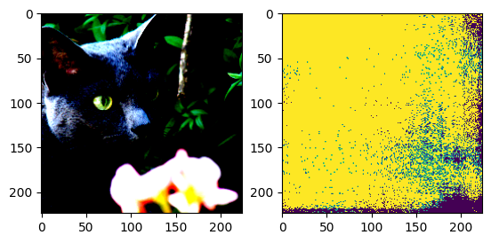
- Inefficient & Ineffective !
Pixel wise classification using image classification
The fully convolutional alternative keeps the classifier structure but applies it densely over the image in one pass, which is far more practical for segmentation.
1 Convolutional VGG
import torchvision.models as models

class ConvolutionalVGG(nn.Module):
    def __init__(self):
        super(ConvolutionalVGG, self).__init__()
        self.features = models.vgg16(pretrained=True).features

        # fc6
        self.fc6 = nn.Conv2d(512, 4096, 7)
        self.relu6 = nn.ReLU(inplace=True)
        self.drop6 = nn.Dropout2d()

        # fc7
        self.fc7 = nn.Conv2d(4096, 4096, 1)
        self.relu7 = nn.ReLU(inplace=True)
        self.drop7 = nn.Dropout2d()

        # fc8
        self.fc8 = nn.Conv2d(4096, 1000, 1)

        self.copy_params_from_vgg16()

    def forward(self, x):
        conv5 = self.features(x)

        fc6 = self.relu6(self.fc6(conv5))
        fc7 = self.drop6(fc6)

        fc7 = self.relu7(self.fc7(fc7))
        fc8 = self.drop7(fc7)

        score = self.fc8(fc8)

        return score

    def copy_params_from_vgg16(self):
        vgg16 = models.vgg16(pretrained=True)
        for i, name in zip([0, 3, 6], ['fc6', 'fc7', 'fc8']):
            l1 = vgg16.classifier[i]
            l2 = getattr(self, name)
            l2.weight.data.copy_(l1.weight.data.view(l2.weight.size()))
            l2.bias.data.copy_(l1.bias.data.view(l2.bias.size()))
conv_vgg = ConvolutionalVGG().cuda()
conv_vgg
ConvolutionalVGG( (features): Sequential( (0): Conv2d(3, 64, kernel_size=(3, 3), stride=(1, 1), padding=(1, 1)) (1): ReLU(inplace=True) (2): Conv2d(64, 64, kernel_size=(3, 3), stride=(1, 1), padding=(1, 1)) (3): ReLU(inplace=True) (4): MaxPool2d(kernel_size=2, stride=2, padding=0, dilation=1, ceil_mode=False) (5): Conv2d(64, 128, kernel_size=(3, 3), stride=(1, 1), padding=(1, 1)) (6): ReLU(inplace=True) (7): Conv2d(128, 128, kernel_size=(3, 3), stride=(1, 1), padding=(1, 1)) (8): ReLU(inplace=True) (9): MaxPool2d(kernel_size=2, stride=2, padding=0, dilation=1, ceil_mode=False) (10): Conv2d(128, 256, kernel_size=(3, 3), stride=(1, 1), padding=(1, 1)) (11): ReLU(inplace=True) (12): Conv2d(256, 256, kernel_size=(3, 3), stride=(1, 1), padding=(1, 1)) (13): ReLU(inplace=True) (14): Conv2d(256, 256, kernel_size=(3, 3), stride=(1, 1), padding=(1, 1)) (15): ReLU(inplace=True) (16): MaxPool2d(kernel_size=2, stride=2, padding=0, dilation=1, ceil_mode=False) (17): Conv2d(256, 512, kernel_size=(3, 3), stride=(1, 1), padding=(1, 1)) (18): ReLU(inplace=True) (19): Conv2d(512, 512, kernel_size=(3, 3), stride=(1, 1), padding=(1, 1)) (20): ReLU(inplace=True) (21): Conv2d(512, 512, kernel_size=(3, 3), stride=(1, 1), padding=(1, 1)) (22): ReLU(inplace=True) (23): MaxPool2d(kernel_size=2, stride=2, padding=0, dilation=1, ceil_mode=False) (24): Conv2d(512, 512, kernel_size=(3, 3), stride=(1, 1), padding=(1, 1)) (25): ReLU(inplace=True) (26): Conv2d(512, 512, kernel_size=(3, 3), stride=(1, 1), padding=(1, 1)) (27): ReLU(inplace=True) (28): Conv2d(512, 512, kernel_size=(3, 3), stride=(1, 1), padding=(1, 1)) (29): ReLU(inplace=True) (30): MaxPool2d(kernel_size=2, stride=2, padding=0, dilation=1, ceil_mode=False) ) (fc6): Conv2d(512, 4096, kernel_size=(7, 7), stride=(1, 1)) (relu6): ReLU(inplace=True) (drop6): Dropout2d(p=0.5, inplace=False) (fc7): Conv2d(4096, 4096, kernel_size=(1, 1), stride=(1, 1)) (relu7): ReLU(inplace=True) (drop7): Dropout2d(p=0.5, inplace=False) (fc8): Conv2d(4096, 1000, kernel_size=(1, 1), stride=(1, 1)) )
transform_conv = transforms.Compose([
    transforms.ToTensor(),
    normalize,
])
test_conv = transform_conv(test_img).cuda().unsqueeze(0)
print(test_conv.size())
conv_out = conv_vgg(test_conv)
pred = torch.argmax(conv_out, dim=1)
pred
tensor([[[285, 285, 284, 284, 284, 284, 285, 285, 285], [284, 284, 284, 284, 284, 284, 285, 285, 285], [284, 284, 284, 284, 284, 284, 287, 287, 287], [285, 284, 285, 284, 284, 284, 284, 287, 287], [285, 285, 285, 285, 285, 285, 287, 287, 285]]], device=‘cuda:0’)
Well…
Although modifying VGG-Net to fully convolutional network results in a pixel-wise ouput, the output resolution is smaller than the original image resolution. Moreover, we can see that many pixels are misclassified (i.e., not 285).
2 Add simple upsampling layer (Bilinear) and retrain with PASCAL VOC 2012
- Re-define the last layer so as to classify classes in the PASCAL VOC datasets
- Use bilinear interpolation to make the network output equal to the input size
import torchvision.models as models

class ConvolutionalVGGwithUpsample(nn.Module):
    def __init__(self):
        super(ConvolutionalVGGwithUpsample, self).__init__()
        self.features = models.vgg16(pretrained=True).features
        self.features[0].padding = (100,100)

        # fc6
        self.fc6 = nn.Conv2d(512, 4096, 7)
        self.relu6 = nn.ReLU(inplace=True)
        self.drop6 = nn.Dropout2d()

        # fc7
        self.fc7 = nn.Conv2d(4096, 4096, 1)
        self.relu7 = nn.ReLU(inplace=True)
        self.drop7 = nn.Dropout2d()

        # fc8
        self.fc8 = nn.Conv2d(4096, 21, 1)

        self.copy_params_from_vgg16()

    def forward(self, x):
        pool5 = self.features(x)

        fc6_out = self.relu6(self.fc6(pool5))
        fc6_out = self.drop6(fc6_out)

        fc7_out = self.relu7(self.fc7(fc6_out))
        fc7_out = self.drop7(fc7_out)

        score = self.fc8(fc7_out)
        score = nn.functional.interpolate(
            score, size=x.shape[-2:], mode='bilinear')  # <-bilinear interpolation

        return score

    def copy_params_from_vgg16(self):
        vgg16 = models.vgg16(pretrained=True)
        for i, name in zip([0, 3], ['fc6', 'fc7']):
            l1 = vgg16.classifier[i]
            l2 = getattr(self, name)
            l2.weight.data.copy_(l1.weight.data.view(l2.weight.size()))
            l2.bias.data.copy_(l1.bias.data.view(l2.bias.size()))
conv_vgg_upsample = ConvolutionalVGGwithUpsample().cuda()
def decode_labels(mask, num_classes=21):
    from PIL import Image
    label_colours = [(0, 0, 0)
                 # 0=background
                 , (128, 0, 0), (0, 128, 0), (128, 128, 0), (0, 0, 128), (128, 0, 128)
                 # 1=aeroplane, 2=bicycle, 3=bird, 4=boat, 5=bottle
                 , (0, 128, 128), (128, 128, 128), (64, 0, 0), (192, 0, 0), (64, 128, 0)
                 # 6=bus, 7=car, 8=cat, 9=chair, 10=cow
                 , (192, 128, 0), (64, 0, 128), (192, 0, 128), (64, 128, 128), (192, 128, 128)
                 # 11=diningtable, 12=dog, 13=horse, 14=motorbike, 15=person
                 , (0, 64, 0), (128, 64, 0), (0, 192, 0), (128, 192, 0), (0, 64, 128)]
                 # 16=potted plant, 17=sheep, 18=sofa, 19=train, 20=tv/monitor

    h, w = mask.shape

    img = Image.new('RGB', (w, h))
    pixels = img.load()
    for j_, j in enumerate(mask[:, :]):
        for k_, k in enumerate(j):
            if k < num_classes:
                pixels[k_, j_] = label_colours[k]
    output = np.array(img)

    return output
model_data = torch.load('../pretrain/lab06/vgg_conv_upsample.pth')
conv_vgg_upsample.load_state_dict(model_data)
with torch.no_grad():
    conv_out = conv_vgg_upsample(test_conv)
output = torch.argmax(conv_out, dim=1)

vis_output = decode_labels(output[0].data.cpu().numpy())
plt.subplot(1,2,1)
plt.imshow(test_conv[0].data.cpu().numpy().transpose((1,2,0)))
plt.subplot(1,2,2)
plt.imshow(vis_output)
Upsampling method with CNNs
1 Transposed Convolution
- The transposed convolution (it is often called as “deconvolution”) is used to up-sample the input resolution by using learnable filters. In contrast to the standard convolution, which aggregates spatial information to a single point, it spreads a point of the input over multiple spatial locations.
- For example, a kernel with a stride of 2 converts a input into a output.
2 Dilated Convolution
-
The dilated convolution introduces ‘a dilation rate’ to the standard convolution.
-
The dilation rate means a spacing value between elements of a kernel, which enlarges the receptive field without introducing additional parameters.
-
For example, a kernel with a dilation rate of 2 has the same receptive field as a kernel while it still use 9 parameters only, compared to the the uses 25 parameters.
Semantic segmentation implementation
FCN8s model
The FCN-8s variant fuses deeper semantic features with shallower skip connections so the final prediction can recover more spatial detail than a single coarse feature map would allow.
Crop boundary example
a = torch.ones((1, 1, 160, 140))
b = torch.ones((1, 1, 120, 120))

try:
    a + b
except:
    print('The size of tensors are different')
    print(a.size())
    print(b.size())

# crop boundary
a = a[:, :, 5: 5+b.size(2), 5:5+b.size(3)]

# add connection with weight
c = 0.01*a + b
-
Predict 1: Conv(in: 4096, out: n_class)
-
Predict 2: Conv(in: 512, out: n_class), weight = 0.01
-
Predict 3: Conv(in: 256, out: n_class), weight = 0.0001
-
Deconv 1: Transposed Conv (in: n_class, out: n_class, stride: 2, biase: False)
-
Deconv 2: Transposed Conv (in: n_class, out: n_class, stride: 2, biase: False)
-
Deconv 3: Transposed Conv (in: n_class, out: n_class, stride: 8, biase: False)
class FCN8s(nn.Module):
    def __init__(self, n_class=21):
        super(FCN8s, self).__init__()
        # VGG features
        self.features = models.vgg16(pretrained=True).features

        # fc6
        self.fc6 = nn.Conv2d(512, 4096, 7)
        self.relu6 = nn.ReLU(inplace=True)
        self.drop6 = nn.Dropout2d()

        # fc7
        self.fc7 = nn.Conv2d(4096, 4096, 1)
        self.relu7 = nn.ReLU(inplace=True)
        self.drop7 = nn.Dropout2d()

        self.pred1 = nn.Conv2d(4096, n_class, 1)
        self.pred2 = nn.Conv2d(512, n_class, 1)  # weight 0.01
        self.pred3 = nn.Conv2d(256, n_class, 1)  # weight 0.0001
        self.deconv1 = nn.ConvTranspose2d(
            in_channels=n_class, out_channels=n_class, kernel_size=4, stride=2, bias=False)
        self.deconv2 = nn.ConvTranspose2d(
            in_channels=n_class, out_channels=n_class, kernel_size=4, stride=2, bias=False)
        self.deconv3 = nn.ConvTranspose2d(
            in_channels=n_class, out_channels=n_class, kernel_size=16, stride=8, bias=False)

        self._initialize_weights()
        self.copy_params_from_vgg16()

    def _initialize_weights(self):
        self.features[0].padding = (100,100)

        for m in self.modules():
            if isinstance(m, nn.MaxPool2d):
                m.ceil_mode=True
            if isinstance(m, nn.ConvTranspose2d):
                assert m.kernel_size[0] == m.kernel_size[1]
                initial_weight = get_upsampling_weight(
                    m.in_channels, m.out_channels, m.kernel_size[0])
                m.weight.data.copy_(initial_weight)

    def forward(self, x):
        input_size = x.shape
        pool_num = 0
        for i, layer in enumerate(self.features):
            x = layer(x)  # ! layer=pool when i=4, 9, 16, 23, 30
            if isinstance(layer, nn.MaxPool2d):
                pool_num += 1
                if pool_num == 3:
                    pool3 = x
                elif pool_num == 4:
                    pool4 = x

        pool5 = x
        # get pool3 > conv > crop to upscore_pool4 > add to upscore_pool4 = fuse_pool3 > deconv=upscore8>crop>softmax
        # get pool4 > conv > crop to up_score2 > add to up_score2 = fuse_pool4 > deconv = upscore_pool4

        # fc6
        fc6_out = self.relu6(self.fc6(pool5))
        fc6_out = self.drop6(fc6_out)

        # fc7
        fc7_out = self.relu7(self.fc7(fc6_out))
        fc7_out = self.drop7(fc7_out)

        # fc8
        score_fr = self.pred1(fc7_out)  # take this and deconv to up_score2
        upscore2 = self.deconv1(score_fr)

        score_pool4 = self.pred2(pool4)
        score_pool4 = score_pool4[:, :, 5: 5 +
                                  upscore2.size(2), 5:5+upscore2.size(3)]
        score_pool4c = 0.01*score_pool4 + upscore2
        fuse_pool4 = upscore2 + score_pool4c
        upscore_pool4 = self.deconv2(fuse_pool4)

        score_pool3 = self.pred3(pool3)
        score_pool3 = score_pool3[:, :, 5: 5 +
                                  upscore_pool4.size(2), 5:5+upscore_pool4.size(3)]
        score_pool3c = 0.0001*score_pool3 + upscore_pool4
        fuse_pool3 = upscore_pool4 + score_pool3c
        upscore8 = self.deconv3(fuse_pool3)

        x = upscore8[:, :, 5: 5 + input_size[2], 5:5+input_size[3]]

        return x

    def copy_params_from_vgg16(self):
        vgg16 = models.vgg16(pretrained=True)
        for i, name in zip([0, 3], ['fc6', 'fc7']):
            l1 = vgg16.classifier[i]
            l2 = getattr(self, name)
            l2.weight.data.copy_(l1.weight.data.view(l2.weight.size()))
            l2.bias.data.copy_(l1.bias.data.view(l2.bias.size()))

def get_upsampling_weight(in_channels, out_channels, kernel_size):
    factor = (kernel_size + 1) // 2
    if kernel_size % 2 == 1:
        center = factor - 1
    else:
        center = factor - 0.5
    og = np.ogrid[:kernel_size, :kernel_size]
    filt = (1 - abs(og[0] - center) / factor) * \
           (1 - abs(og[1] - center) / factor)
    weight = np.zeros((in_channels, out_channels, kernel_size, kernel_size),
                      dtype=np.float64)
    weight[range(in_channels), range(out_channels), :, :] = filt
    return torch.from_numpy(weight).float()
model = FCN8s().cuda()
Data Loader functions
import random
import os

def read_file(path_to_file):
    with open(path_to_file) as f:
        img_list = []
        for line in f:
            img_list.append(line[:-1])
    return img_list

def chunker(seq, size):
    return (seq[pos:pos + size] for pos in range(0, len(seq), size))

def flip(I, flip_p):
    if flip_p > 0.5:
        return np.fliplr(I)
    else:
        return I

def scale_im(img_temp, scale):
    new_dims = (int(img_temp.shape[0] * scale), int(img_temp.shape[1] * scale))
    return cv2.resize(img_temp, new_dims).astype(float)

def get_data(chunk, gt_path='../dataset-dllab/lab06/gt', img_path='../dataset-dllab/lab06/img'):
    assert len(chunk) == 1

    scale = random.uniform(0.5, 1.3)
    flip_p = random.uniform(0, 1)

    images = cv2.imread(os.path.join(img_path, chunk[0] + '.jpg')).astype(float)

    images = cv2.resize(images, (321, 321)).astype(float)
    images = scale_im(images, scale)
    images[:, :, 0] = images[:, :, 0] - 104.008
    images[:, :, 1] = images[:, :, 1] - 116.669
    images[:, :, 2] = images[:, :, 2] - 122.675
    images = flip(images, flip_p)
    images = images[:, :, :, np.newaxis]
    images = images.transpose((3, 2, 0, 1))
    images = torch.from_numpy(images.copy()).float()

    gt = cv2.imread(os.path.join(gt_path, chunk[0] + '.png'))[:, :, 0]
    gt[gt == 255] = 0
    gt = flip(gt, flip_p)

    dim = int(321 * scale)

    gt = cv2.resize(gt, (dim, dim), interpolation=cv2.INTER_NEAREST).astype(float)

    labels = gt[np.newaxis, :].copy()

    return images, labels
Data load
img_list = read_file('../dataset-dllab/lab06/list/train_aug.txt')
data_list = []

for i in range(10):
    np.random.shuffle(img_list)
    data_list.extend(img_list)
data_gen = chunker(data_list, 1)
lr =  1e-5  # choose your lr

optimizer = optim.Adam(model.parameters(), lr=lr)
optimizer.zero_grad()
max_iter = 20000
Training loop and loss tracking
- Use a cross-entropy loss.
- Print a training loss for every 100 iterations.
- Show that the training loss steadily decreases.
def loss_calc(out, label):
    criterion = nn.CrossEntropyLoss()
    return criterion(out, label)
running_loss = 0.0

for iter in range(max_iter + 1):
    inputs, label = get_data(next(data_gen))

    # change label to torch
    label = torch.from_numpy(label.copy()).type(torch.LongTensor)
    # move to GPU
    inputs = inputs.cuda()  # torch.Size([1, 3, 321, 321])
    label = label.cuda()  # numpy.ndarray(1, 321, 321)

    # Initialize gradients
    optimizer.zero_grad()

    # Forward
    out = model(inputs)

    # Calculate loss
    loss = loss_calc(out, label)
    running_loss += loss/100

    # Backward
    loss.backward()

    # Update weights
    optimizer.step()

    # Logging
    if iter == 0:
        best = 100
    elif iter % 100 == 0:
        print(f'Iteration: {iter}, Loss: {running_loss}')
        if best > running_loss:
            best = running_loss
            torch.save(model, f"./weights/best.pth")
        # torch.save(model, f"./weights/iter{iter}_lomodel = ss{running_loss}.pth")
        history = running_loss
        running_loss = 0
torch.save(model, f"./weights/last.pth")
Results and discussion
- The evaluation section reports both quantitative and qualitative results so the segmentation quality is visible in the metrics and in the predicted masks.
- The
validation_miouhelper computes mean IoU and provides a concrete reference point; in this run the trained model clears the 0.47 mIoU baseline from the example setup. - The
decode_labelhelper converts predicted class maps into colorized masks for qualitative inspection.
def validation_miou(model):
    max_label = 20
    hist = np.zeros((max_label + 1, max_label + 1))

    def fast_hist(a, b, n):
        k = (a >= 0) & (a < n)
        return np.bincount(n * a[k].astype(int) + b[k], minlength=n ** 2).reshape(n, n)

    val_list = open('../dataset-dllab/lab06/list/val.txt').readlines()

    with torch.no_grad():
        for idx, i in enumerate(val_list):
            print('{}/{} ...'.format(idx + 1, len(val_list)))

            img = cv2.imread(os.path.join('../dataset-dllab/lab06/img', i[:-1] + '.jpg')).astype(float)

            img[:, :, 0] -= 104.008
            img[:, :, 1] -= 116.669
            img[:, :, 2] -= 122.675

            data = torch.from_numpy(img.transpose((2,0,1))).float().cuda().unsqueeze(0)
            score = model(data)

            output = score.cpu().data[0].numpy().transpose(1, 2, 0)
            output = np.argmax(output, axis=2)
            gt = cv2.imread(os.path.join('../dataset-dllab/lab06/gt', i[:-1] + '.png'), 0)

            hist += fast_hist(gt.flatten(), output.flatten(), max_label + 1)

        miou = np.diag(hist) / (hist.sum(1) + hist.sum(0) - np.diag(hist))
        print("Mean iou = ", np.sum(miou) / len(miou))

    return np.sum(miou) / len(miou)
model = torch.load("./weights/last.pth")

#mIoU of model
fcn8s_miou= validation_miou(model)

#mIoU of model in section 1.2.2
bilinearVgg_miou=validation_miou(
    conv_vgg_upsample)
print('Mean IoU of model FCN-8s is:', fcn8s_miou)
print('Mean IoU of model bilinear upsampled VGG-16 is:', bilinearVgg_miou)
# Visualize the result
with torch.no_grad():
    conv_out = model(test_conv)  # ! inference
output = torch.argmax(conv_out, dim=1)

vis_output = decode_labels(output[0].data.cpu().numpy())
plt.subplot(1, 2, 1)
plt.imshow(test_conv[0].data.cpu().numpy().transpose((1, 2, 0)))
plt.subplot(1, 2, 2)
plt.imshow(vis_output)
plt.show()
References
[1] FCN official code (https://github.com/shelhamer/fcn.berkeleyvision.org)
[2] Upsampling method (https://towardsdatascience.com/types-of-convolutions-in-deep-learning-717013397f4d)
[3] Cs231n (http://cs231n.stanford.edu/slides/2017/cs231n_2017_lecture11.pdf)
Discussion
The FCN-8s run was a clear improvement over the bilinear-upsampled VGG baseline, even though it still fell short of the target mIoU.
Quantitative analysis
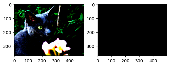
The mIoU of bilinear sampled VGG-16 was 0.03, but for FCN-8s achieved 0.35. That is still below the target of 0.47, but the gap seems tied to the notebook setup and pretrained weights rather than to the FCN conversion alone. The bilinear VGG baseline was especially unstable at inference time, which appears to be related to dropout behavior in the provided weights. Given the server issues around the original environment, a damaged or inconsistent checkpoint is also plausible.
Qualitative analysis
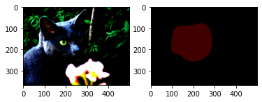
The final visualization separates the cat region from the background, with black for class 0 and red for class 8. Earlier outputs were almost entirely background, so the final mask at least shows that the network learned the basic foreground structure.