Building FSRCNN From Scratch for Real-Time Super-Resolution

May 18, 2026

EEE4423

EEE4423 FSRCNN Super Resolution Low-Level Vision PyTorch

Paper Context

The background reading focused on why FSRCNN was a practical improvement over the earlier SRCNN line of work. The original insight was not just to get better super-resolution quality, but to reorganize the computation so most of the network runs in low-resolution space and only upsamples at the end with a learned deconvolution layer.

That tradeoff between quality and runtime is what makes FSRCNN worth implementing. The code is organized around shrinking, mapping, expanding, and deconvolution because each stage helps move most of the computation into low-resolution space.

Implementation Walkthrough

The sections below walk through the FSRCNN blocks, the training setup, and the final super-resolution results.

Super-resolution with CNN

What is super-resolution?

Image super-resolution is a technique which enhances an image quality in terms of spatial resolution.

Low Resolution (LR) Image : Pixel density within an image is small, hence it offers few details.

High Resolution (HR) Image : Pixel density within an image is large, hence it offers a lot of details.

Super-resolution reconstructs a high-resolution image (with restored details) from a low-resolution image.

Why deep learning?

Learning based methods outperform simple interpolations or hand-designed methods.

Simple Interpolations : Easy to implement (e.g., bicubic), but give poor visual quality, since the details are hard to be preserved.

Hand-designed methods : Involve several steps (e.g., sparse coding and dictionary learning), but not all of them can be optimized.

Deep learning (CNN) : Steps in the hand-designed methods can be combined into one big step with all of its parts being optimizable.

SRCNN and FSRCNN

One of the pioneering works using CNNs to solve the super-resolution task.

SRCNN

Starts with a bicubic-upsampled image.

Convolutions are performed to improve a quality of the image.

FSRCNN

Starts with a low-resolution image. (Hence faster.)

Convolutions are performed in low-resolution spaces followed by a deconvolution which enhances spatial resolution.

Deconvolution ( $\equiv$ Transposed Convolution)

How to do deconvolution?

Given a $4\times4$ input, we can generate a $6\times6$ output by using a $3\times3$ filter.
Warning! : It is not an actual deconvolution! It just mimics the deconvolution by filter learning.
(We suggest you to use the terminology “transposed convolution” instead.)

Why is it called as transposed convolution?

In order to generate a single pixel in the output, the input pixels are aggregated by a flipped version of the filter.

The reason why we call convolving with flipped filter as a transposed convolution is described here:
https://towardsdatascience.com/up-sampling-with-transposed-convolution-9ae4f2df52d0.
TL;DR : When we define a convolution operation by a matrix multiplication between a filter matrix and an input vector, then going backward (i.e., generating an input from an output) can be expressed by a matrix multiplication between transpose of the filter matrix and an output vector.

How to interpret it as a convolution?

Conv2d with flipped filter, given that (filter size - 1) zeros are padded along borders
$\equiv$ ConvTranspose2d with no padding

Then, what does the padding mean in the transposed convolution?

It is not an actual padding. It works reversely, that is, it decreases the spatial size of the output.

Note. On the other hand, the argument output_padding in ConvTranspose2d increases the spatial size of the output.
See https://pytorch.org/docs/master/nn.html#torch.nn.ConvTranspose2d for details.

Lastly, how does a stride work in the transposed convolution?

The stride is applied on the output space. It mainly determines a factor of increasing.
We can interpret it as a Conv2d with flipped filter, given that (stride - 1) zeros are padded between input pixels.

Implementing FSRCNN

Dataset

91-image dataset.

Augmented with scaling / roatation / flipping.

Use only Y channel of YCbCr color space.

64x64 HR image patches.

Scaling factor = 4.

Network architecture

FSRCNN (d,s,m) = (56,12,4), following the standard shrinking, mapping, expanding, and deconvolution layout from the paper.

PReLU activations.

Deconvolution at the last layer (without activation).
The input resolution is $16\times16$ and the output resolution is $64\times64$ , in case of scale factor 4.
The implementation requires selecting appropriate arguments (padding, stride, and output_padding) for ConvTranspose2d.

Loss function

Mean squared error (MSE) loss between estimation & ground-truth:
${1\over N} \sum^{N}_{i=1} \lVert F(Y^{i};\theta) - X^{i} \rVert^{2}_{2}$ .

Training

Weight initialization.
Convolutional weights : ~ $N(0,0.02^2)$ (Different from the paper, but for simplicity).
Convolutional biases : Zero initialization.
Deconvolutional weights : ~ $N(0,0.001^2)$ .
Deconvolutional biases : Zero initialization.

Learning rate.
Convolutional parameters : $10^{-3}$ .
Deconvolutional parameters : $10^{-4}$ .

Optimizer.
Adam optimizer with default parameters ( $\beta_{1} = 0.9, \beta_{2} = 0.999$ ).
(Note. The paper proposes to use the SGD optimizer, but using the Adam optimizer shows faster convergence.)

51 epochs without learning rate scheduling.

Evaluation metric

Peak Signal-to-Noise Ratio (PSNR) : $10 \log_{10} \left( MAX_{I} \over MSE \right)$ .

Measured with Y channel of images.

References

[1] https://cv-tricks.com/deep-learning-2/image-super-resolution-to-enhance-photos/
[2] https://deepsense.ai/using-deep-learning-for-single-image-super-resolution/
[3] Dong et al., “Learning a deep convolutional network for image super-resolution”, ECCV, 2014.
[4] Dong et al., “Accelerating the super-resolution convolutional neural network”, ECCV, 2016.
[5] https://medium.com/apache-mxnet/transposed-convolutions-explained-with-ms-excel-52d13030c7e8
[6] https://pytorch.org/docs/master/nn.html#torch.nn.ConvTranspose2d

FSRCNN with PyTorch

import torch
import torch.nn as nn
from torch.utils.data.dataset import Dataset
import matplotlib.pyplot as plt

from misc.lab05.imresize import imresize
import numpy as np
import skimage
import os
import glob
from skimage.io import imread
import skimage

os.environ["CUDA_VISIBLE_DEVICES"]="0"

Data loader


class T91_images(Dataset):
    def __init__(self, data_dir = "../dataset/lab05/HR_patches_from_T91.npy", HR_patch_size = 64, scale_factor = 4):
        super(T91_images, self).__init__()
        self.HR_patches_np = np.load(data_dir) # pre-processed patches
        self.HR_patch_size = HR_patch_size
        self.scale_factor = scale_factor

    def __getitem__(self, idx):
        HR_patch_np = self.HR_patches_np[idx] # high resolution patch
        LR_patch_np = imresize(HR_patch_np, scalar_scale = 1.0 / self.scale_factor) # low resolution patch
        BC_patch_np = imresize(LR_patch_np, scalar_scale = self.scale_factor) # bicubic upsampled patch

        HR_patch = torch.from_numpy(HR_patch_np).type(torch.FloatTensor)
        LR_patch = torch.from_numpy(LR_patch_np).type(torch.FloatTensor)
        BC_patch = torch.from_numpy(BC_patch_np).type(torch.FloatTensor)

        HR_patch = HR_patch.unsqueeze(0) # size : 1(c) x 64(h) x 64(w)
        LR_patch = LR_patch.unsqueeze(0) # size : 1(c) x 16(h) x 16(w)
        BC_patch = BC_patch.unsqueeze(0) # size : 1(c) x 64(h) x 64(w)

        return HR_patch, LR_patch, BC_patch # Y-channel patches

    def __len__(self):
        return len(self.HR_patches_np)

class Set5(Dataset):
    def __init__(self, data_dir = '../dataset/lab05/Set5/', scale_factor=4):
        super(Set5, self).__init__()
        self.image_filenames = [os.path.join(data_dir, x) for x in sorted(os.listdir(data_dir))]
        self.scale_factor = scale_factor

    def load_img(self, filepath):
        img = skimage.io.imread(filepath)
        ch = img.ndim
        if ch == 2:
            img = skimage.color.gray2rgb(img)
        img = skimage.color.rgb2ycbcr(img)

        return img / 255.

    def calculate_valid_crop_size(self, crop_size, scale_factor):
        return crop_size - (crop_size % scale_factor)

    def __getitem__(self, idx):
        # load image
        img_np = self.load_img(self.image_filenames[idx])

        # original HR image size
        h, w, _ = img_np.shape

        # determine valid HR image size with scale factor
        HR_img_w = self.calculate_valid_crop_size(w, self.scale_factor)
        HR_img_h = self.calculate_valid_crop_size(h, self.scale_factor)

        # determine lr_img LR image size
        LR_img_w = HR_img_w // self.scale_factor
        LR_img_h = HR_img_h // self.scale_factor

        HR_img_np = img_np[:HR_img_h,:HR_img_w,:] # high resolution image
        LR_img_np = imresize(HR_img_np, scalar_scale = 1.0/self.scale_factor) # low resolution image
        BC_img_np = imresize(LR_img_np, scalar_scale = self.scale_factor) # bicubic upsampled image

        HR_img = torch.from_numpy(HR_img_np).type(torch.FloatTensor).permute(2,0,1) # size : 3(c) x h x w
        LR_img = torch.from_numpy(LR_img_np).type(torch.FloatTensor).permute(2,0,1) # size : 3(c) x (h/scale_factor) x (w/scale_factor)
        BC_img = torch.from_numpy(BC_img_np).type(torch.FloatTensor).permute(2,0,1) # size : 3(c) x h x w

        return HR_img, LR_img, BC_img # YCbCr images

    def __len__(self):
        return len(self.image_filenames)


scale_factor = 4 # 1/4 down scaling

train_dataset = T91_images(data_dir = "../dataset/lab05/HR_patches_from_T91.npy", HR_patch_size = 64, scale_factor = scale_factor)
test_dataset = Set5(data_dir = "../dataset/lab05/Set5/", scale_factor = scale_factor)

train_loader = torch.utils.data.DataLoader(dataset = train_dataset,
                                           batch_size = 64,
                                           shuffle = True, num_workers = 4)
test_loader = torch.utils.data.DataLoader(dataset = test_dataset,
                                          batch_size = 1,
                                          shuffle = False)

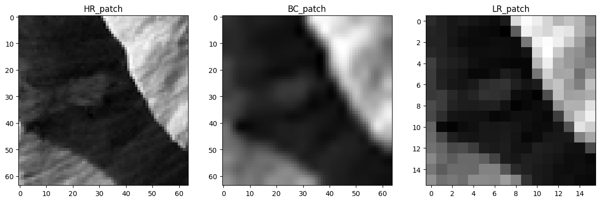
Visualize a training sample

(HR_patch, LR_patch, BC_patch) = train_dataset[100]
fig = plt.figure(figsize=(15,5))
ax1 = fig.add_subplot(1, 3, 1)
ax2 = fig.add_subplot(1, 3, 2)
ax3 = fig.add_subplot(1, 3, 3)
ax1.imshow(HR_patch.squeeze(0).numpy(), cmap='gray')
ax1.set_title("HR_patch")
ax2.imshow(BC_patch.squeeze(0).numpy(), cmap='gray')
ax2.set_title("BC_patch")
ax3.imshow(LR_patch.squeeze(0).numpy(), cmap='gray')
ax3.set_title("LR_patch")
plt.show()

png

FSRCNN model


class FSRCNN(nn.Module):
    def __init__(self, scale_factor = 4):
        super(FSRCNN, self).__init__()
        '''
        padding? = zero padding according to filter size [ref 4.1]
        bias? = True, specified
        norm? = False, only min-max norm for output layer to 0 to 1
        '''

        self.scale_factor = scale_factor
        self.d = 56
        self.s = 12
        self.m = 4

        # Feature extraction
        self.feature_extraction = nn.Sequential(
            nn.Conv2d(1, self.d, 5, padding=2),  # Conv(5,d,1)
            nn.PReLU(),  # one learnable param
        )

        # shrinking
        self.shrinking = nn.Sequential(
            nn.Conv2d(self.d, self.s, 1),  # Conv(1,s,d)
            nn.PReLU(),  # one learnable param
        )

        # non-linear mapping
        self.non_lin_mapping = nn.Sequential(
            # maybe better to interate the layer append m times
            nn.Conv2d(self.s, self.s, 3, padding=1),  # Conv(3, s, s)
            nn.PReLU(),  # one learnable param
            nn.Conv2d(self.s, self.s, 3, padding=1),  # Conv(3, s, s)
            nn.PReLU(),  # one learnable param
            nn.Conv2d(self.s, self.s, 3, padding=1),  # Conv(3, s, s)
            nn.PReLU(),  # one learnable param
            nn.Conv2d(self.s, self.s, 3, padding=1),  # Conv(3, s, s)
            nn.PReLU(),  # one learnable param
        )

        # expanding
        self.expanding = nn.Sequential(
            nn.Conv2d(self.s, self.d, 1),  # Conv(1, d, s)
            nn.PReLU(),  # one learnable param
        )

        # deconv
        self.deconvolution = nn.ConvTranspose2d(
            self.d, 1, 9, stride=self.scale_factor, padding=3, output_padding=1)  # DeConv(9, 1, s)

    def weight_init(self):
        for m in self.modules():
            if isinstance(m, nn.Conv2d):
                nn.init.normal_(m.weight.data, mean = 0.0, std = 0.02)
#                 nn.init.kaiming_normal_(m.weight.data, a=0.25) # for SGD
                if m.bias is not None:
                    m.bias.data.zero_()
            if isinstance(m, nn.ConvTranspose2d):
                nn.init.normal_(m.weight.data, mean = 0.0, std = 0.001)
                if m.bias is not None:
                    m.bias.data.zero_()

    def forward(self, LR_patch):

        x1 = self.feature_extraction(LR_patch)  # B, d, H, W
        x2 = self.shrinking(x1)  # B, s, H, W
        x3 = self.non_lin_mapping(x2)  # B, s, H, W
        x4 = self.expanding(x3)  # B, d, H, W
        output = self.deconvolution(x4)  # B, 1, 4H, 4W

        # Normalize output to [0,1]
        test_img_size = output.shape  # (batch, y_channel, H, W)
        output = output.view(test_img_size[0], -1)  # (batch, y_channel, H * W)
        output -= output.min(dim=1, keepdim=True)[0]
        output /= output.max(dim=1, keepdim=True)[0]
        output = output.view(*test_img_size)  # (batch, y_channel, H, W)

        return output


model = FSRCNN(scale_factor = scale_factor)
model.weight_init()
num_total_params = sum(p.numel() for p in model.parameters())
print("The number of parameters : ", num_total_params)

#  USE GPU FOR MODEL  #
device = torch.device("cuda:0" if torch.cuda.is_available() else "cpu")
model.to(device)


lr_conv = 1e-3
lr_deconv = 1e-4
# momentum = 0.9

param_conv = list(model.feature_extraction.parameters())+\
             list(model.shrinking.parameters())+\
             list(model.non_lin_mapping.parameters())+\
             list(model.expanding.parameters())

param_deconv = model.deconvolution.parameters()

# optimizer = torch.optim.SGD([{'params':param_conv},
#                              {'params':param_deconv, 'lr':lr_deconv}],
#                              lr = lr_conv, momentum = momentum)

optimizer = torch.optim.Adam([{'params':param_conv},
                             {'params':param_deconv, 'lr':lr_deconv}],
                             lr = lr_conv)

Training the FSRCNN model and tracking PSNR

import time

criterion = nn.MSELoss()

if not os.path.exists("./weights/"):
    os.mkdir("./weights/")

if not os.path.exists("./weights/lab05/"):
    os.mkdir("./weights/lab05/")

num_epochs = 51

def PSNR(pred, gt, s = 0): # input images : 0~1 normalized / s : scale factor
    if pred.is_cuda:
        pred = pred.cpu()
    if gt.is_cuda:
        gt = gt.cpu()
    pred = pred[:,:,s:-s,s:-s] # shave border
    gt = gt[:,:,s:-s,s:-s]
    pred = pred.clamp(0, 1)
    diff = pred - gt
    mse = np.mean(diff.numpy() ** 2)
    if mse == 0:
        return 100
    return 10 * np.log10(1.0 / mse)

for epoch in range(num_epochs):
    # training stage
    model.train()
    total_loss = 0
    start = time.time()
    for i, (HR_patch, LR_patch, BC_patch) in enumerate(train_loader):

        # Load to gpu
        HR_patch = HR_patch.to(device)
        LR_patch = LR_patch.to(device)

        # Forward
        output = model(LR_patch)
        loss = criterion(output, HR_patch)
        total_loss += loss

        # Backward
        optimizer.zero_grad()
        loss.backward()
        optimizer.step()

    # test stage
    end = time.time()
    model.eval()

    # Calculate PSNR
    total_psnr = 0
    total_psnr_bic = 0
    # Iterate through test dataset
    with torch.no_grad():
        for (HR_img, LR_img, BC_img) in test_loader:
            # need to select only the "Y" channel from "YCbCr"

            # Load to gpu (only "Y" channel)
            HR_img = HR_img[:, 0:1, :, :].to(device)
            LR_img = LR_img[:, 0:1, :, :].to(device)
            BC_img = BC_img[:, 0:1, :, :].to(device)

            # Forward
            output = model(LR_img)

            # Metrics : PSNR
            total_psnr += PSNR(output, HR_img, s=scale_factor) / \
                len(test_loader)  # FSRCNN
            total_psnr_bic += PSNR(BC_img, HR_img,
                                   s=scale_factor)/len(test_loader)  # Bicubic

        # Print Loss
        print('Epochs: {0}. Loss: {1:.6f}. PSNR: {2:.3f} (bicubic)\t{3:.3f} (FSRCNN)\tElapsed time: {4} sec'.format(epoch, total_loss / (i+1), total_psnr_bic, total_psnr, end-start))

    # save weights
    if epoch % 5 == 0 and epoch != 0:
        torch.save({'state_dict':model.state_dict()},'./weights/lab05/checkpoint_%03d.pkl'%(epoch))

Visual comparison on RGB test examples

def ycbcr2rgb(im): # input image : ranges from 0 to 255
    xform = np.array([[1, 0, 1.402], [1, -0.34414, -.71414], [1, 1.772, 0]])
    rgb = im.astype(np.float32) # np.float is depreciated from numpy version 1.24
    rgb[:,:,[1,2]] -= 128
    rgb = rgb.dot(xform.T)
    np.putmask(rgb, rgb > 255, 255)
    np.putmask(rgb, rgb < 0, 0)
    return np.uint8(rgb)

trained_weight = torch.load("./weights/lab05/checkpoint_050.pkl")
model.load_state_dict(trained_weight['state_dict'])
model.eval()

with torch.no_grad():
    for (HR_img, LR_img, BC_img) in test_loader:
        # need to select only the "Y" channel from "YCbCr"

        # Load to gpu (only "Y" channel)
        LR_y = LR_img[:, 0:1, :, :].to(device)
        BC_cbcr = BC_img[:, 1:3, :, :].to(device)

        # Forward
        output = model(LR_y)
        FSRCNN_img = torch.cat((output, BC_cbcr), dim=1).to('cpu') # back to cpu

        HR_img = ycbcr2rgb(HR_img.squeeze(0).permute(1, 2, 0).numpy() * 255)
        LR_img = ycbcr2rgb(LR_img.squeeze(0).permute(1, 2, 0).numpy() * 255)
        BC_img = ycbcr2rgb(BC_img.squeeze(0).permute(1, 2, 0).numpy() * 255)
        FSRCNN_img = ycbcr2rgb(FSRCNN_img.squeeze(0).permute(1, 2, 0).numpy() * 255)
        fig = plt.figure(figsize=(10, 10))
        ax1 = fig.add_subplot(2, 2, 1)
        ax2 = fig.add_subplot(2, 2, 2)
        ax3 = fig.add_subplot(2, 2, 3)
        ax4 = fig.add_subplot(2, 2, 4)
        ax1.imshow(HR_img)
        ax1.set_title("HR_img")
        ax2.imshow(BC_img)
        ax2.set_title("BC_img")
        ax3.imshow(LR_img)
        ax3.set_title("LR_img")
        ax4.imshow(FSRCNN_img)
        ax4.set_title("FSRCNN")
        plt.show()

png

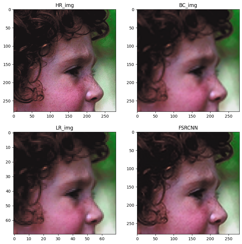
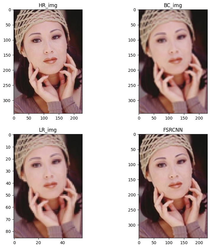
Discussion

This implementation follows the $FSRCNN(56,12,4)$ setting fairly closely, with a few practical deviations such as Adam instead of SGD, no $(n-1)$ -pixel crop during training, and different feature-map sizes driven by the dataset setup.

Qualitative analysis

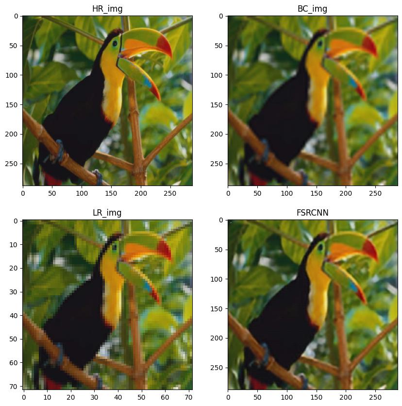
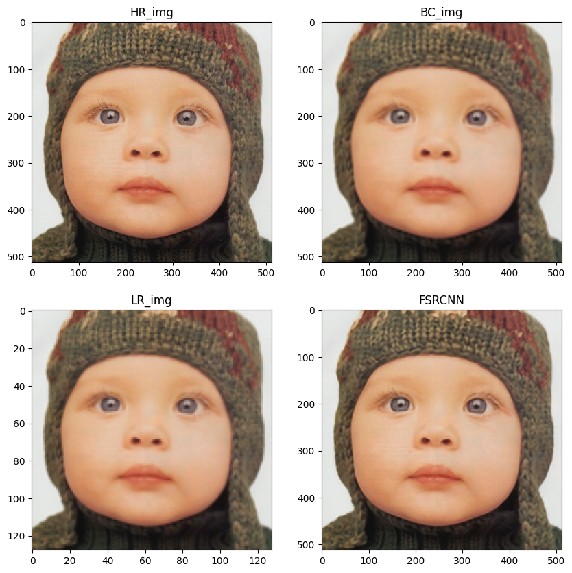
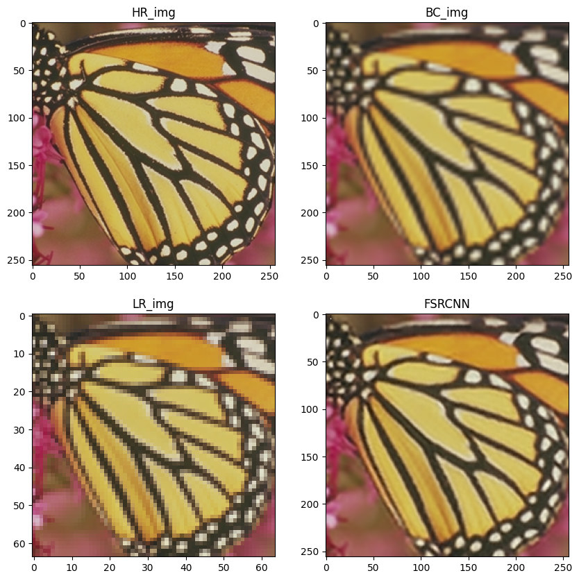
The visualization results show the performance improvement even visible to human eye. Although still blurry compared to the original image, more of high frequency features were restored and aliasing was reduced.

Quantitative analysis

The training log shows a steady PSNR improvement over bicubic interpolation, even though the notebook setup did not include a separate best-checkpoint selection step.

The run reached 30.245 PSNR, below the 30.71 reported for $FSRCNN(56,12,4)$ on Set5 x4, but still well above the 28.432 bicubic baseline. Much of that gap is explained by the different training recipe: the paper uses a two-stage schedule with the 91-image dataset followed by General-100 fine-tuning.