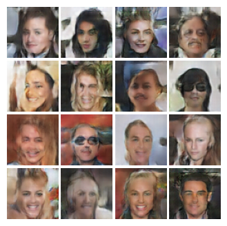
Building DCGAN From Scratch for Face Generation
Paper Context
The background reading started from the original GAN objective and then moved into the practical design rules introduced by DCGAN. The basic adversarial game between generator and discriminator is elegant, but unstable in practice; DCGAN became influential because it showed that a small set of architectural constraints could make convolutional GAN training much more reliable.
Those constraints are also what made the implementation practical. Once the generator and discriminator were built with strided convolutions, batch normalization, and the usual activation choices, the training behavior became much easier to reason about.
Implementation Walkthrough
The sections below focus on the model definitions, the adversarial training loop, and the generated samples from the run.
Implementation for DCGAN
1. Dataset
- CelebA dataset
- Resize to (64, 64)
2. Network architecture
Architecture Guideline
Generative model G
Xavier initialization (Glorot & Bengio [2])
It makes sure the weights to keep the propagation in a reasonable range through many layers
Use nn.init.xavier_uniform_ for the Xavier initialization
(The authors suggested a proper initialization for DCGAN training, but the xavier initialization also works well)Latent vector Z for input (size=100)
(In this implementation it is reshaped to (bs, 100, 1, 1) for upconvolution.)The original discussion referenced stride 5 upconvolutions, while this implementation uses stride 4.
Batch normalization is applied to every layer except the last one
Discriminative model D
Xavier Initialization
Real data or fake data for input (size=64x64)
It’s structure is the reverse version of the generative model G where the upconvolutions are replaced to convolutions and the last output size is changed to (bs, 1, 1, 1)
Use the batch normalization except for the last layer
3. Loss function
- Discriminative model D
- Binary cross entropy loss for the real data
- Binary cross entropy loss for the fake data
()
- Generative model G
- Binary cross entropy loss for the real data (It is actually fake)
()
4. Training Strategy
- Same as the GAN training algorithm
- The generative model G and the discriminative model D are trained alternatively during training
- When the parameters of the model D are being updated, the back-propagation in the model G is blocked
DCGAN with PyTorch
import os
import random
import torch
import torch.nn as nn
import torch.nn.parallel
import torch.utils.data
import torchvision
import torchvision.datasets as dset
import torchvision.transforms as transforms
import numpy as np
import matplotlib.pyplot as plt
import matplotlib.gridspec as gridspec
import os
import os.path as osp

%matplotlib inline

os.environ["CUDA_DEVICE_ORDER"]="PCI_BUS_ID"
os.environ["CUDA_VISIBLE_DEVICES"]="0"
Parameter Setting
- The key training hyperparameters are collected here for the run shown below
# Data root directory
data_root = '../dataset-dllab/lab13/celebA/'

# Batch size during training
bs = 128

# Size of image size
img_size = 64

# Channels of generator feature
gfc = 64

# Channels of discriminator feature
dfc = 64

# Size of latent vector z
z_size = 100

# Number of training epochs
num_epochs = 5

# Learning rate for optimizing
lr = 0.0002

# Beta1 hyperparameter for Adam optimizers
beta1 = 0.5

# Real or Fake label
real_label = 1
fake_label = 0
transform = transforms.Compose([
    transforms.Resize(img_size),
    transforms.CenterCrop(img_size),
    transforms.ToTensor(),
    transforms.Normalize((0.5, 0.5, 0.5), (0.5, 0.5, 0.5))])

dataset = dset.ImageFolder(root=data_root,
                           transform=transform)
data_loader = torch.utils.data.DataLoader(dataset=dataset,
                                           batch_size=bs,
                                           shuffle=True,
                                           drop_last=True)
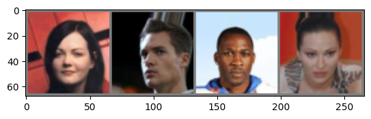
Visualize a few images
def imshow(inp, title=None):
    """Imshow for Tensor."""
    inp = inp.numpy().transpose((1, 2, 0))
    mean = np.array([0.5, 0.5, 0.5])
    std = np.array([0.5, 0.5, 0.5])
    inp = std * inp + mean
    inp = np.clip(inp, 0, 1)
    plt.imshow(inp)
    if title is not None:
        plt.title(title)
    plt.pause(0.001)  # pause a bit so that plots are updated
data_loader_sample = torch.utils.data.DataLoader(dataset=dataset,
                                                 batch_size=4,
                                                 shuffle=True)

# Get a batch of training data
inputs, classes = next(iter(data_loader_sample))

# Make a grid from batch
out = torchvision.utils.make_grid(inputs)

imshow(out)
Utils
- The helper below factors out the repeated convolution and upconvolution blocks used throughout the model
def conv2d(params_list, batch_norm = True):
    channel_in, channel_out, kernel_size, stride, padding, activation = params_list
    layers = []
    if batch_norm:
        layers += [nn.Conv2d(channel_in, channel_out, kernel_size, stride, padding, bias=False),
                   nn.BatchNorm2d(channel_out)]
        nn.init.xavier_uniform_(layers[0].weight)
    else:
        layers += [nn.Conv2d(channel_in, channel_out, kernel_size, stride, padding, bias=False)]
        nn.init.xavier_uniform_(layers[0].weight)

    if activation == 'ReLU':
        layers += [nn.ReLU(inplace=True)]
    if activation == 'LeakyReLU':
        layers += [nn.LeakyReLU(0.2, inplace=True)]
    if activation == 'Tanh':
        layers += [nn.Tanh()]
    if activation == 'Sigmoid':
        layers += [nn.Sigmoid()]

    return nn.Sequential(*layers)

def upconv2d(params_list, batch_norm = True):
    channel_in, channel_out, kernel_size, stride, padding, activation = params_list
    layers = []
    if batch_norm:
        layers += [nn.ConvTranspose2d(channel_in, channel_out, kernel_size, stride, padding, bias=False),
                   nn.BatchNorm2d(channel_out)]
        nn.init.xavier_uniform_(layers[0].weight)
    else:
        layers += [nn.ConvTranspose2d(channel_in, channel_out, kernel_size, stride, padding, bias=False)]
        nn.init.xavier_uniform_(layers[0].weight)

    if activation == 'ReLU':
        layers += [nn.ReLU(inplace=True)]
    if activation == 'LeakyReLU':
        layers += [nn.LeakyReLU(0.2, inplace=True)]
    if activation == 'Tanh':
        layers += [nn.Tanh()]
    if activation == 'Sigmoid':
        layers += [nn.Sigmoid()]

    return nn.Sequential(*layers)
Generator
- The
cfg_glist specifies the upconvolution blocks used in the generator - The activation field accepts
'ReLU','LeakyReLU','Tanh', and'Sigmoid' - An empty string disables the activation branch when a layer should stay linear
- Padding and stride choices follow the standard convolution arithmetic
(See https://pytorch.org/docs/stable/nn.html) - Each block is constructed with the conv2d() and upconv2d() helpers defined above
# [input channels, output channels, kernel_size, strides, paddings, activation fuctions]
cfg_g = [[100, 512, 4, 1, 0, 'ReLU'],
         [512, 256, 4, 2, 1, 'ReLU'],
         [256, 128, 4, 2, 1, 'ReLU'],
         [128, 64, 4, 2, 1, 'ReLU'],
         [64, 3, 4, 2, 1, 'Tanh']]

class Generator(nn.Module):
    def __init__(self):
        super(Generator, self).__init__()

        # The generator has multiple sequential blocks called upconv#, created using the upconv2d function defined above.
        # It takes the configuration of list as an input.
        # Here we can use the nested list of configurations for each upconv# layer.
        self.upconv1 = upconv2d(cfg_g[0], batch_norm = True)
        self.upconv2 = upconv2d(cfg_g[1], batch_norm = True)
        self.upconv3 = upconv2d(cfg_g[2], batch_norm = True)
        self.upconv4 = upconv2d(cfg_g[3], batch_norm = True)
        self.upconv5 = upconv2d(cfg_g[4], batch_norm = False)

    def forward(self, x):

        # input x.shape = bs, 100, 1, 1
        # All the upconv blocks are sequentially connected.
        x = self.upconv1(x)
        x = self.upconv2(x)
        x = self.upconv3(x)
        x = self.upconv4(x)
        x = self.upconv5(x)
        # output x.shape = bs, 3, 64, 64
        return x
Discriminator
- The
cfg_dlist specifies the convolution blocks used in the discriminator - The activation field accepts
'ReLU','LeakyReLU','Tanh', and'Sigmoid' - An empty string disables the activation branch when a layer should stay linear
- Padding and stride choices follow the standard convolution arithmetic
(See https://pytorch.org/docs/stable/nn.html) - Each block is constructed with the conv2d() and upconv2d() helpers defined above
# [input channels, output channels, kernel_size, strides, paddings, activation fuctions]
cfg_d = [[3, 64, 4, 2, 1, 'LeakyReLU'],
         [64, 128, 4, 2, 1, 'LeakyReLU'],
         [128, 256, 4, 2, 1, 'LeakyReLU'],
         [256, 512, 4, 2, 1, 'LeakyReLU'],
         [512, 1, 4, 1, 0, 'Sigmoid']]

class Discriminator(nn.Module):
    def __init__(self):
        super(Discriminator, self).__init__()

        # The discriminator has multiple sequential blocks called conv#, created using the conv2d function defined above.
        # It takes the configuration of list as an input.
        # Here we can use the nested list of configurations for each conv# layer.
        self.conv1 = conv2d(cfg_d[0], batch_norm = True)
        self.conv2 = conv2d(cfg_d[1], batch_norm = True)
        self.conv3 = conv2d(cfg_d[2], batch_norm = True)
        self.conv4 = conv2d(cfg_d[3], batch_norm = True)
        self.conv5 = conv2d(cfg_d[4], batch_norm = False)

    def forward(self, x):

        # input x.shape = bs, 3, 64, 64
        # All the conv blocks are sequentially connected.
        x = self.conv1(x)
        x = self.conv2(x)
        x = self.conv3(x)
        x = self.conv4(x)
        x = self.conv5(x)
        # output x.shape = bs, 100, 1, 1
        return x
model_G = Generator()
model_D = Discriminator()

#  USE GPU FOR MODEL  #

device = torch.device("cuda:0" if torch.cuda.is_available() else "cpu")
model_G.to(device)
print(model_G)
model_D.to(device)
criterion = nn.BCELoss()

optimizer_G = torch.optim.Adam(model_G.parameters(), lr=lr, betas=(beta1, 0.999))
optimizer_D = torch.optim.Adam(model_D.parameters(), lr=lr, betas=(beta1, 0.999))
Training the DCGAN
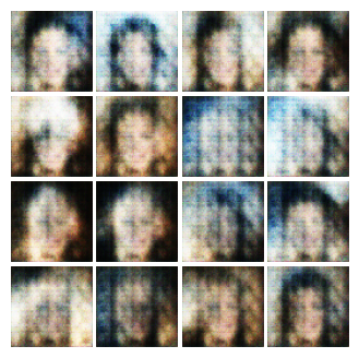
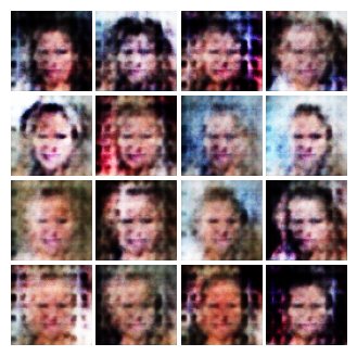
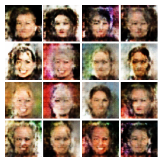
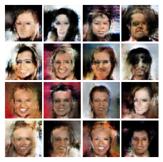
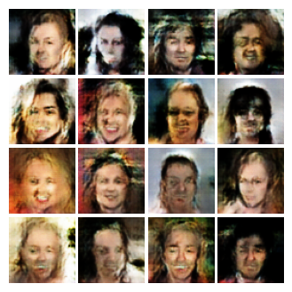
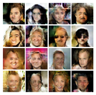
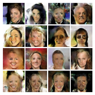
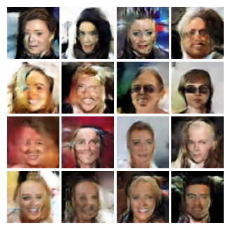
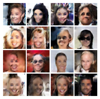
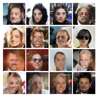
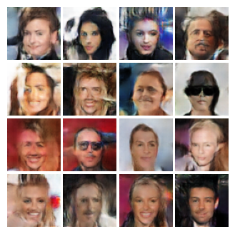
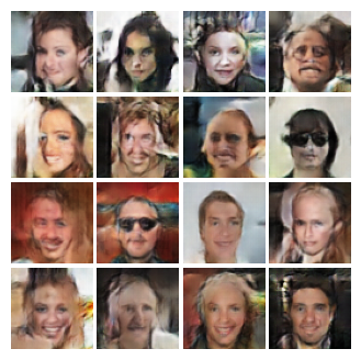
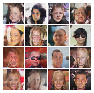
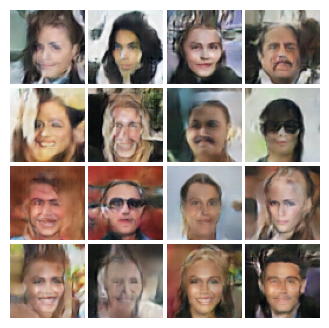
- The training loop below is followed by generated samples for qualitative inspection.
- Sample quality serves as the main qualitative indicator for this run.
def plot(samples):
    fig = plt.figure(figsize=(4, 4))
    gs = gridspec.GridSpec(4, 4)
    gs.update(wspace=0.05, hspace=0.05)
    for i, sample in enumerate(samples):
        ax = plt.subplot(gs[i])
        plt.axis('off')
        ax.set_xticklabels([])
        ax.set_yticklabels([])
        ax.set_aspect('equal')
        plt.imshow(sample.reshape(64, 64, 3), cmap='Greys_r')
    return fig

label_real = torch.full((bs,), real_label, device=device, dtype=torch.float)
label_fake = torch.full((bs,), fake_label, device=device, dtype=torch.float)

#  The input noise for inference
fixed_noise = torch.randn(bs, z_size, 1, 1, device=device, dtype=torch.float)

for epoch in range(num_epochs):

    model_G.train()
    model_D.train()

    for i, data in enumerate(data_loader):

        data = data[0].to(device)

        ### Update discriminator model

        # Clear gradients w.r.t. parameters
        model_D.zero_grad()

        # Forward pass to get results of discriminator for real data
        output_D_real = model_D(data).view(-1)

        # Calculate Loss
        err_D_real = criterion(output_D_real, label_real)

        # Generating noise inputs for generating fake samples
        noise = torch.randn(bs, z_size, 1, 1, device=device)

        # Forward pass to get generated samples
        output_G = model_G(noise)

        # Forward pass to get results of discriminator for fake data
        output_D_fake = model_D(output_G.detach()).view(-1)

        # Calculate Loss
        err_D_fake = criterion(output_D_fake, label_fake)

        # Combine the losses for real data and fake data
        err_D = err_D_real + err_D_fake

        # Getting gradients w.r.t. parameters
        err_D.backward()

        # Updating parameters
        optimizer_D.step()

        ### Update generator model

        # Clear gradients w.r.t. parameters
        model_G.zero_grad()

        # Forward pass to get results of discriminator for fake data
        output_G_real = model_D(output_G).view(-1)

        # Calculate Loss
        err_G = criterion(output_G_real, label_real)

        # Getting gradients w.r.t. parameters
        err_G.backward()

        # Updating parameters
        optimizer_G.step()

        # Output training stats
        if i % 400 == 0 and i != 0:
            print('[%d/%d][%d/%d]\tLoss_D: %.4f\tLoss_G: %.4f\t'
                  % (epoch, num_epochs, i, len(data_loader),
                     err_D.item(), err_G.item()))

            model_G.eval()
            model_D.eval()
            with torch.no_grad():
                output = model_G(fixed_noise).detach().cpu().numpy()
                output = np.transpose((output+1)/2, (0, 2, 3, 1))
                fig = plot(output[:16])

            model_G.train()
            model_D.train()
References
[1] Radford et al., “Unsupervised Representation Learning with Deep Convolutional Generative Adversarial network”, ICLR, 2016.
[2] Glorot & Bengio, “Understanding the difficulty of training deep feedforward neural networks”, AISTATS 2010
Discussion
The sample images were much more informative than the raw loss curves in this run.
Quantitative analysis
The generator and discriminator were implemented directly from the stated configurations, using the provided conv2d and upconv2d helpers for the convolution blocks. During training, the two losses kept oscillating, which is typical for GANs, even while the sample images improved visually.
Qualitative analysis
The visual progression is clearer than the loss curves: early outputs are mostly noisy blobs, then faces gradually emerge as the generator learns enough of the dataset statistics to fool the discriminator.
One clear limitation of plain DCGAN is the lack of control over the generated content, which is exactly why later variants such as conditional GANs and image-to-image models became so important.