Building CycleGAN From Scratch for Unpaired Image Translation
Paper Context
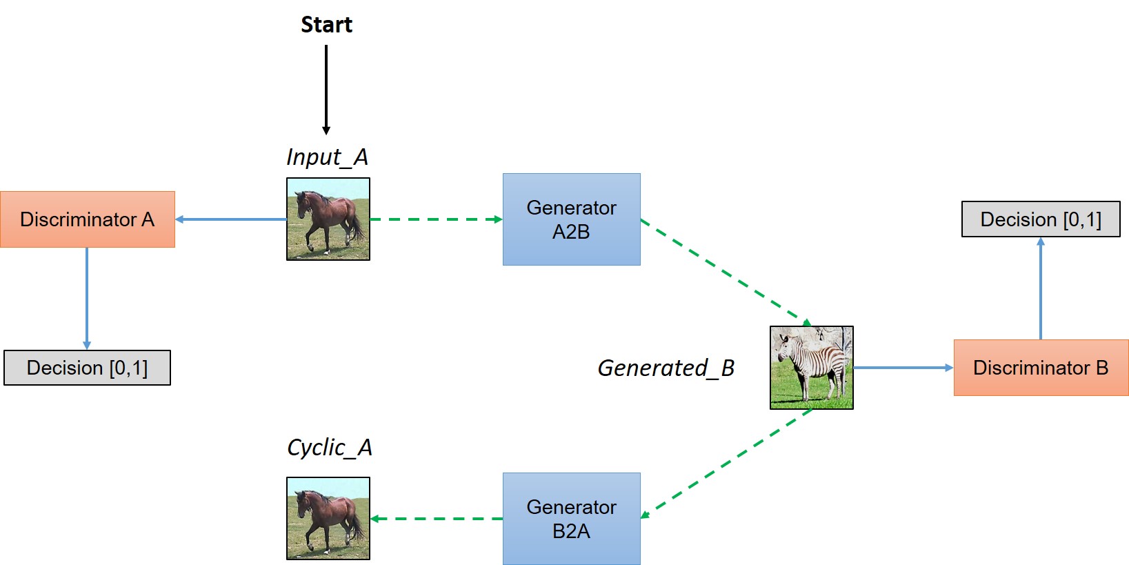
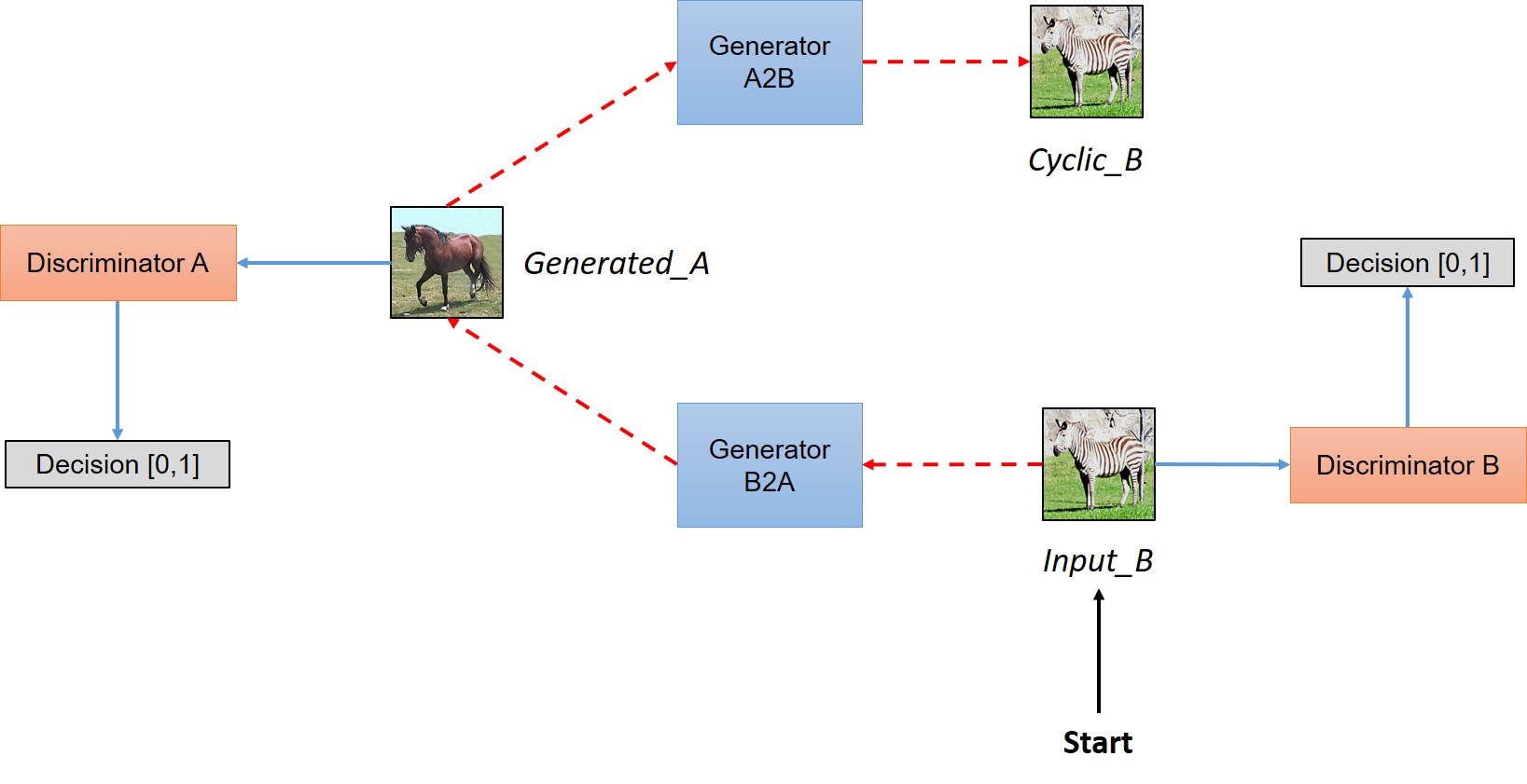
The background reading emphasized why CycleGAN was a meaningful break from earlier conditional GAN setups. Paired image translation methods like pix2pix assume aligned input-output pairs, but many realistic translation problems do not come with such supervision. CycleGAN replaces that requirement with a structural constraint: if a model maps domain A to domain B, then mapping the result back to A should reconstruct the original sample.
That cycle-consistency constraint is the part that gives the implementation its shape. Most of the work goes into keeping the translation tied closely enough to the source image that the model does not drift into arbitrary texture transfer.
Implementation Walkthrough
The sections below cover the generator-discriminator setup, the cycle loss, and the translation results from the experiment.
Implementation for CycleGAN
- Cycle GAN leverages a cycle consistency in image-to-image translation
- Unlike a conditional GAN, the cycle GAN considers unpaired training data
1. Dataset
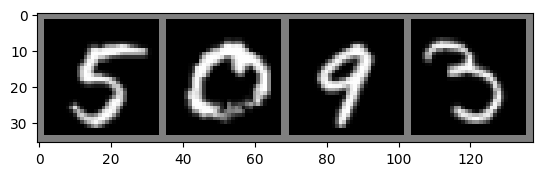
- MNIST dataset
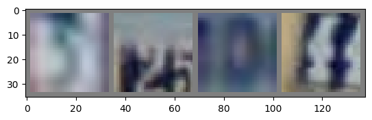
- SVHN dataset
- Note that the MNIST data is gray, where the number of the channel is 1
2. Network architecture
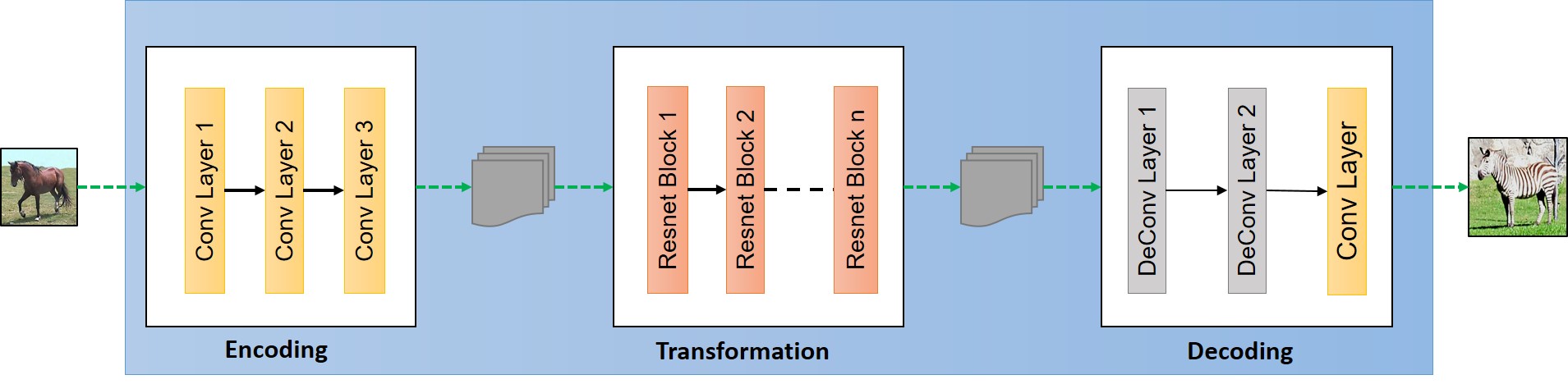
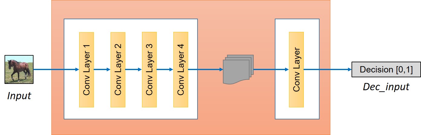
- Overall architecture
Generative model G
Xavier initialization (Glorot & Bengio [3])
It makes sure the weights to keep the propagation in a reasonable range through many layers
Use
nn.init.xavier_uniform_for the Xavier initializationThe generative model has three components:
- Encoder:
Convolutional network for feature extracting
2 convolutional layers and 2 LeakyReLU activations
The output channel sizes are 64, 128 respectively
The kernel size of the convolutional layers are 7 and 3, respectively
(Other size choices are possible, but these dimensions are the ones used in this implementation.)All the strides are 2
Batch normalization is applied to every encoder layer except the first one
- Transformer:
Learn how it would like to transform the feature vector of and image from A to B.
The transformer uses ResNet blocks with skip connections between input and output for feature transformation
(Please refer to He et al.[3])3 resnet block layers and each of layer is followed by LeakyReLU activation
All the output channel sizes are 128
All the kernel sizes and strides are 3 and 1, respectively
- Decoder:
Upconvolutional network for reconstructing an image
2 upconvolutional layers, one LeakyReLU activations, and one Tanh activation which is for the last layer
The output channel sizes are 128, 64, and 3, respectively for the SVHN data, and 128, 64, and 1, respectively for the MNIST data
All the kernel sizes and strides are 4 and 2, respectively
Batch normalization is applied throughout the decoder except at the final output layer
Discriminative model D
Xavier Initialization
It contains 4 convolutional layers, 3 LeakyReLU activations, and one Sigmoid activation which is for the last layer
The output channel sizes are 64, 128, 256, and 1, respectively
All the kernel sizes are 4 except for the last kernel size which is 1
The strides from the first two layers are 2 and the rest of them are 1
Batch normalization([4]) is applied to the discriminator except at the first and last layers
3. Loss function
(In the paper, the authors use the L2 loss for the GAN loss, but the binary cross entropy loss also works well)
- Discriminative model and
- The loss for is followed as
- Binary cross entropy loss for the real data
- Binary cross entropy loss for the fake data
- The loss for is followed as
- Binary cross entropy loss for the real data
- Binary cross entropy loss for the fake data
()
( is the generator where translate to and vice versa)
Generative model and
Binary cross entropy loss for the real data (It is actually fake)
()
- The cycle loss for measuring difference between and and vice versa
Cycle GAN with Pytorch
import os
import os.path as osp
import random
import torch
import torch.nn as nn
import torch.nn.parallel
import torch.nn.functional as F
import torch.backends.cudnn as cudnn
import torch.utils.data
import torchvision
import torchvision.datasets as dset
import torchvision.transforms as transforms
import numpy as np
import matplotlib.pyplot as plt
import time

%matplotlib inline

os.environ["CUDA_DEVICE_ORDER"]="PCI_BUS_ID"
os.environ["CUDA_VISIBLE_DEVICES"]="0"
Parameter Setting
- The key training hyperparameters are collected here for the run shown below
# Data root directory
train_X_root = '../dataset-dllab/lab14/mnist/'
train_Y_root = '../dataset-dllab/lab14/svhn/'

# Weight save directory
vis_num = 2
save_dir = './weights/lab14/cyclegan'
if not osp.exists(save_dir):
    os.makedirs(save_dir)

# Batch size during training
bs = 64

# Size of image
img_height = 32
img_width = 32
img_size = 32
img_channel = 3

# Channels of generator feature
gfc = 64

# Channels of discriminator feature
dfc = 64

# Number of training epochs
num_epochs = 5

# Learning rate for optimizing
lr = 0.0002

# Beta1 hyperparameter for Adam optimizers
beta1 = 0.5

# Real or Fake label
real_label = 1
fake_label = 0
transform_1ch = transforms.Compose([
    transforms.Resize(img_size),
    transforms.ToTensor(),
    transforms.Normalize((0.5,), (0.5,))])

transform_3ch = transforms.Compose([
    transforms.Resize(img_size),
    transforms.ToTensor(),
    transforms.Normalize((0.5, 0.5, 0.5), (0.5, 0.5, 0.5))])

train_X_set = dset.MNIST(root=train_X_root,
                         train=True,
                         transform=transform_1ch,
                         download=False)
train_Y_set = dset.SVHN(root=train_Y_root,
                        split='train',
                        transform=transform_3ch,
                        download=False)
test_X_set = dset.MNIST(root=train_X_root,
                         train=False,
                         transform=transform_1ch,
                         download=False)
test_Y_set = dset.SVHN(root=train_Y_root,
                        split='test',
                        transform=transform_3ch,
                        download=False)
train_X_loader = torch.utils.data.DataLoader(train_X_set,
                                             batch_size=bs,
                                             shuffle=True,
                                             drop_last=True)

train_Y_loader = torch.utils.data.DataLoader(train_Y_set,
                                             batch_size=bs,
                                             shuffle=True,
                                             drop_last=True)

test_X_loader = torch.utils.data.DataLoader(test_X_set,
                                             batch_size=bs,
                                             shuffle=False,
                                             drop_last=True)

test_Y_loader = torch.utils.data.DataLoader(test_Y_set,
                                             batch_size=bs,
                                             shuffle=False,
                                             drop_last=True)
Visualize a few images
def imshow(inp, title=None):
    """Imshow for Tensor."""
    inp = inp.numpy().transpose((1, 2, 0))
    mean = np.array([0.5, 0.5, 0.5])
    std = np.array([0.5, 0.5, 0.5])
    inp = std * inp + mean
    inp = np.clip(inp, 0, 1)
    plt.imshow(inp)
    if title is not None:
        plt.title(title)
    plt.pause(0.001)  # pause a bit so that plots are updated
data_loader_X_sample = torch.utils.data.DataLoader(train_X_set,
                                                 batch_size=4,
                                                 shuffle=True)
data_loader_Y_sample = torch.utils.data.DataLoader(train_Y_set,
                                                 batch_size=4,
                                                 shuffle=True)

# Get a batch of training data
X = next(iter(data_loader_X_sample))
Y = next(iter(data_loader_Y_sample))

# Make a grid from batch
out_X = torchvision.utils.make_grid(X[0])
out_Y = torchvision.utils.make_grid(Y[0])

imshow(out_X)
imshow(out_Y)
Utils
- The helper below factors out the repeated convolution and upconvolution blocks used throughout the model
References
[1] Zhu et al., “Unpaired Image-to-Image Translation using Cycle-Consistent Adversarial Networks”, ICCV, 2017.
[2] https://hardikbansal.github.io/CycleGANBlog/
[3] Glorot & Bengio, “Understanding the difficulty of training deep feedforward neural networks”, AISTATS 2010.
[4] Ioffe & Szegedy, “Batch Normalization: Accelerating Deep Network Training by Reducing Internal Covariate Shift”, ICML 2015.
def conv2d(params_list, batch_norm = True):
    channel_in, channel_out, kernel_size, stride, padding, activation = params_list
    layers = []
    if batch_norm:
        layers += [nn.Conv2d(channel_in, channel_out, kernel_size, stride, padding, bias=False),
                   nn.BatchNorm2d(channel_out)]
        nn.init.xavier_uniform_(layers[0].weight)
    else:
        layers += [nn.Conv2d(channel_in, channel_out, kernel_size, stride, padding, bias=False)]
        nn.init.xavier_uniform_(layers[0].weight)

    if activation.lower() == 'relu':
        layers += [nn.ReLU(inplace=True)]
    if activation.lower() == 'leakyrelu':
        layers += [nn.LeakyReLU(0.2, inplace=True)]
    if activation.lower() == 'tanh':
        layers += [nn.Tanh()]
    if activation.lower() == 'sigmoid':
        layers += [nn.Sigmoid()]

    return nn.Sequential(*layers)

def upconv2d(params_list, batch_norm = True):
    channel_in, channel_out, kernel_size, stride, padding, activation = params_list
    layers = []
    if batch_norm:
        layers += [nn.ConvTranspose2d(channel_in, channel_out, kernel_size, stride, padding, bias=False),
                   nn.BatchNorm2d(channel_out)]
        nn.init.xavier_uniform_(layers[0].weight)
    else:
        layers += [nn.ConvTranspose2d(channel_in, channel_out, kernel_size, stride, padding, bias=False)]
        nn.init.xavier_uniform_(layers[0].weight)

    if activation.lower() == 'relu':
        layers += [nn.ReLU(inplace=True)]
    if activation.lower() == 'leakyrelu':
        layers += [nn.LeakyReLU(0.2, inplace=True)]
    if activation.lower() == 'tanh':
        layers += [nn.Tanh()]
    if activation.lower() == 'sigmoid':
        layers += [nn.Sigmoid()]

    return nn.Sequential(*layers)

def transpose(ndarray):
    return np.transpose(ndarray, [0,2,3,1])

def gray2rgb(ndarray):
    return np.concatenate((ndarray, ndarray, ndarray), axis=2)
Generator
- The generator configuration lists specify the encoder, transformer, and decoder blocks
- The activation field accepts
'ReLU','LeakyReLU','Tanh', and'Sigmoid' - An empty string disables the activation branch when a layer should stay linear
- Padding and stride choices follow the standard convolution arithmetic
(See https://pytorch.org/docs/stable/nn.html) - Each block is constructed with the conv2d() and upconv2d() helpers defined above
# [input channels, output channels, kernel_size, strides, paddings]

cfg_g_enc_X = [[3, 64, 7, 2, 3, 'LeakyReLU'], # No batchnorm
               [64, 128, 3, 2, 1, 'LeakyReLU']]
cfg_g_enc_Y = [[3, 64, 7, 2, 3, 'LeakyReLU'], # No batchnorm
               [64, 128, 3, 2, 1, 'LeakyReLU']]
cfg_g_trans = [[128, 128, 3, 1, 1, 'LeakyReLU'],
               [128, 128, 3, 1, 1, 'LeakyReLU'],
               [128, 128, 3, 1, 1, 'LeakyReLU']]
cfg_g_dec_X = [[128, 64, 4, 2, 1, 'LeakyReLU'],
               [64, 3, 4, 2, 1, 'tanh']] # No batchnorm
cfg_g_dec_Y = [[128, 64, 4, 2, 1, 'LeakyReLU'],
               [64, 1, 4, 2, 1, 'tanh']] # No batchnorm

class Generator_X(nn.Module):
    def __init__(self):
        super(Generator_X, self).__init__()

        # MNIST to SVHN
        # encoder
        self.conv1 = conv2d(cfg_g_enc_X[0], batch_norm = False)
        self.conv2 = conv2d(cfg_g_enc_X[1], batch_norm = True)

        # transformer
        self.trans1 = conv2d(cfg_g_trans[0], batch_norm = True)
        self.trans2 = conv2d(cfg_g_trans[1], batch_norm = True)
        self.trans3 = conv2d(cfg_g_trans[2], batch_norm = True)

        # decoder
        self.upconv1 = upconv2d(cfg_g_dec_X[0], batch_norm = True)
        self.upconv2 = upconv2d(cfg_g_dec_X[1], batch_norm = False)

    def forward(self, x):

        # channel manipulation
        # utilizing predefined gray2rgb and transpose functions
        x = x.cpu()
        x = x.detach().numpy()
        x = transpose(x)
        x = transpose(x)
        x = gray2rgb(x)
        x = transpose(x)
        x = torch.tensor(x).to(torch.device("cuda:0" if torch.cuda.is_available() else "cpu"))
        # x.shape = B, 3(c), H, W

        # encoder
        e = self.conv1(x)
        e = self.conv2(e)

        # transformer
        t = self.trans1(e)
        t = self.trans2(t)
        t = self.trans3(t)
        r = t + e #residual connection

        # decoder
        d = self.upconv1(r)
        d = self.upconv2(d)

        return d

class Generator_Y(nn.Module):
    def __init__(self):
        super(Generator_Y, self).__init__()

        # SVHN to MNIST
        # encoder
        self.conv1 = conv2d(cfg_g_enc_Y[0], batch_norm = False)
        self.conv2 = conv2d(cfg_g_enc_Y[1], batch_norm = True)

        # transformer
        self.trans1 = conv2d(cfg_g_trans[0], batch_norm = True)
        self.trans2 = conv2d(cfg_g_trans[1], batch_norm = True)
        self.trans3 = conv2d(cfg_g_trans[2], batch_norm = True)

        # decoder
        self.upconv1 = upconv2d(cfg_g_dec_Y[0], batch_norm = True)
        self.upconv2 = upconv2d(cfg_g_dec_Y[1], batch_norm = False)

    def forward(self, x):

        # encoder
        e = self.conv1(x)
        e = self.conv2(e)

        # transformer
        t = self.trans1(e)
        t = self.trans2(t)
        t = self.trans3(t)
        r = t + e #residual connection

        # decoder
        d = self.upconv1(r)
        d = self.upconv2(d)

        return d
Discriminator
- The discriminator configuration lists specify the convolution blocks used for each domain
- The activation field accepts
'ReLU','LeakyReLU','Tanh', and'Sigmoid' - An empty string disables the activation branch when a layer should stay linear
- Padding and stride choices follow the standard convolution arithmetic
(See https://pytorch.org/docs/stable/nn.html) - Each block is constructed with the conv2d() and upconv2d() helpers defined above
# [input channels, output channels, kernel_size, strides, paddings]

cfg_d_X = [[3, 64, 4, 2, 1, 'LeakyReLU'], # No batchnorm
           [64, 128, 4, 2, 0, 'LeakyReLU'],
           [128, 256, 4, 1, 2, 'LeakyReLU'],
           [256, 1, 1, 1, 0, 'Sigmoid']] # No batchnorm
cfg_d_Y = [[3, 64, 4, 2, 1, 'LeakyReLU'], # No batchnorm
           [64, 128, 4, 2, 0, 'LeakyReLU'],
           [128, 256, 4, 1, 2, 'LeakyReLU'],
           [256, 1, 1, 1, 0, 'Sigmoid']] # No batchnorm

class Discriminator_X(nn.Module):
    def __init__(self):
        super(Discriminator_X, self).__init__()

        # MNIST to score
        self.conv1 = conv2d(cfg_d_X[0], batch_norm = False)
        self.conv2 = conv2d(cfg_d_X[1], batch_norm = True)
        self.conv3 = conv2d(cfg_d_X[2], batch_norm = True)
        self.conv4 = conv2d(cfg_d_X[3], batch_norm = False)

    def forward(self, x):

        # channel manipulation
        # utilizing predefined gray2rgb and transpose functions
        x = x.cpu()
        x = x.detach().numpy()
        x = transpose(x)
        x = transpose(x)
        x = gray2rgb(x)
        x = transpose(x)
        x = torch.tensor(x).to(torch.device("cuda:0" if torch.cuda.is_available() else "cpu"))
        # x.shape = B, 3(c), H, W

        x = self.conv1(x)
        x = self.conv2(x)
        x = self.conv3(x)
        x = self.conv4(x)

        return x

class Discriminator_Y(nn.Module):
    def __init__(self):
        super(Discriminator_Y, self).__init__()

        # SHVN to score
        self.conv1 = conv2d(cfg_d_Y[0], batch_norm = False)
        self.conv2 = conv2d(cfg_d_Y[1], batch_norm = True)
        self.conv3 = conv2d(cfg_d_Y[2], batch_norm = True)
        self.conv4 = conv2d(cfg_d_Y[3], batch_norm = False)

    def forward(self, x):

        x = self.conv1(x)
        x = self.conv2(x)
        x = self.conv3(x)
        x = self.conv4(x)

        return x
model_G_X = Generator_X()
model_G_Y = Generator_Y()
model_D_X = Discriminator_X()
model_D_Y = Discriminator_Y()

#  USE GPU FOR MODEL  #

device = torch.device("cuda:0" if torch.cuda.is_available() else "cpu")
model_G_X.to(device)
print(model_G_X)
model_G_Y.to(device)
print(model_G_Y)
model_D_X.to(device)
print(model_D_X)
model_D_Y.to(device)
criterion_GAN = nn.BCELoss()
criterion_L1 = nn.L1Loss()

optimizer_G_X = torch.optim.Adam(model_G_X.parameters(), lr=lr, betas=(beta1, 0.999))
optimizer_G_Y = torch.optim.Adam(model_G_Y.parameters(), lr=lr, betas=(beta1, 0.999))
optimizer_D_X = torch.optim.Adam(model_D_X.parameters(), lr=lr, betas=(beta1, 0.999))
optimizer_D_Y = torch.optim.Adam(model_D_Y.parameters(), lr=lr, betas=(beta1, 0.999))
Training the CycleGAN
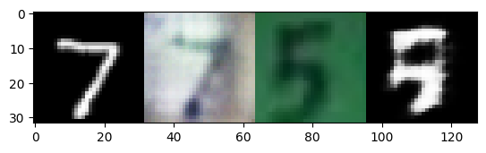
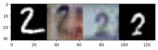
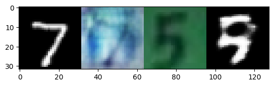
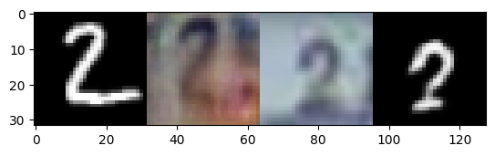
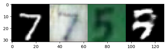
- The training run below ends with generated sample outputs for qualitative inspection.
- Sample quality is treated here as the main qualitative check on the translation behavior.
label_real = torch.full((bs, 1, 8, 8), real_label, dtype=torch.float32, device=device)
label_fake = torch.full((bs, 1, 8, 8), fake_label, dtype=torch.float32, device=device)

num_iter = 0
max_iter = num_epochs*len(train_X_loader)

train_start_time = time.time()
for epoch in range(1, num_epochs+1):
    for batch_index, data_X in enumerate(train_X_loader):
        model_G_X.train()
        model_G_Y.train()
        model_D_X.train()
        model_D_Y.train()

        data_X = data_X[0].to(device)
        data_Y = next(iter(train_Y_loader))[0].to(device)

        ### Update discriminator model

        # data_X = MNIST, data_Y = SVHN
        # data_x -> G_X => gen_X
        # gen_Y <= G_Y <- data_Y
        #  V                 V
        # D_X               D_Y

        # reset gradients
        optimizer_D_X.zero_grad()
        optimizer_D_Y.zero_grad()

        # G forward
        gen_Y = model_G_X(data_X)
        gen_X = model_G_Y(data_Y)

        # D forward gen
        pred_gen_X = model_D_X(gen_X.detach())
        pred_gen_Y = model_D_Y(gen_Y.detach())

        # D forward data
        pred_data_X = model_D_X(data_X)
        pred_data_Y = model_D_Y(data_Y)

        # D_X loss
        loss_D_gen_X = criterion_GAN(pred_gen_X, label_fake)
        loss_D_data_X = criterion_GAN(pred_data_X, label_real)
        loss_D_X = loss_D_gen_X + loss_D_data_X

        # D_Y loss
        loss_D_gen_Y = criterion_GAN(pred_gen_Y, label_fake)
        loss_D_data_Y = criterion_GAN(pred_data_Y, label_real)
        loss_D_Y = loss_D_gen_Y + loss_D_data_Y

        # full D loss
        loss_D = loss_D_X + loss_D_Y

        # backward pass
        loss_D.backward()

        # update parameters
        optimizer_D_X.step()
        optimizer_D_Y.step()

        err_D = loss_D

        ### Update generator model

        # reset gradients
        model_G_X.zero_grad()
        model_G_Y.zero_grad()

        # D forward gen
        pred_gen_X = model_D_X(gen_X)
        pred_gen_Y = model_D_Y(gen_Y)

        # G loss
        loss_G_X = criterion_GAN(pred_gen_Y, label_real)
        loss_G_Y = criterion_GAN(pred_gen_X, label_real)

        # reverse G forward
        cycle_X = model_G_Y(gen_Y)
        cycle_Y = model_G_X(gen_X)

        # cycle loss
        loss_cycle_X = criterion_L1(cycle_X, data_X)
        loss_cycle_Y = criterion_L1(cycle_Y, data_Y)

        cycle_importance = 10.0 # authors set lambda to 10 for all experiments.
        loss_C = loss_cycle_X + loss_cycle_Y
        loss_G = loss_G_X + loss_G_Y + cycle_importance*loss_C

        # backward pass
        loss_G.backward()

        # update parameters
        optimizer_G_X.step()
        optimizer_G_Y.step()

        err_G = loss_G

        err_C = loss_C

        num_iter += 1
        # Output training stats
        if num_iter%100 == 0:
            print('it[{:04d}/{:04d}] \tLoss_D:{:.4f} \tLoss_G:{:.4f} \tLoss_C:{:.4f} \telapsed_time:{:.2f}mins'.format(
                num_iter, max_iter, err_D.item(), err_G.item(), err_C.item(), (time.time()-train_start_time)/60
            ))

        if num_iter%1000==0 or num_iter==max_iter:
            save_name = osp.join(save_dir, 'it{:04d}.pt'.format(num_iter))
            torch.save({
                'model_G_X': model_G_X.state_dict(),
                'model_G_Y': model_G_Y.state_dict()
            }, save_name)

            with torch.no_grad():
                model_G_X.eval()
                model_G_Y.eval()
                for test_index, data_X in enumerate(test_X_loader):
                    if test_index == 0:

                        data_X = data_X[0].to(device)
                        data_Y = next(iter(test_Y_loader))[0].to(device)

                        output_X = model_G_X(data_X)
                        output_Y = model_G_Y(data_Y)

                        data_X = ((data_X+1)/2).cpu().data.numpy()
                        data_Y = ((data_Y+1)/2).cpu().data.numpy()

                        output_X = ((output_X + 1)/2).cpu().data.numpy()
                        output_Y = ((output_Y + 1)/2).cpu().data.numpy()

                        for vis_idx in range(vis_num):
                            data_X_, data_Y_ = gray2rgb(transpose(data_X)[vis_idx]), transpose(data_Y)[vis_idx]
                            output_X_, output_Y_  = transpose(output_X)[vis_idx], gray2rgb(transpose(output_Y)[vis_idx])
                            outputs = np.concatenate((data_X_, output_X_, data_Y_, output_Y_), axis=1)
                            plt.imshow(outputs)
                            plt.pause(0.001)
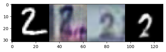
it[1100/4685] Loss_D:1.1743 Loss_G:6.9200 Loss_C:0.2183 elapsed_time:0.67mins it[1200/4685] Loss_D:1.0362 Loss_G:6.5731 Loss_C:0.1939 elapsed_time:0.73mins it[1300/4685] Loss_D:1.0615 Loss_G:6.3587 Loss_C:0.1994 elapsed_time:0.79mins it[1400/4685] Loss_D:1.1764 Loss_G:7.2305 Loss_C:0.2156 elapsed_time:0.85mins it[1500/4685] Loss_D:1.1320 Loss_G:7.1352 Loss_C:0.1977 elapsed_time:0.90mins it[1600/4685] Loss_D:1.2638 Loss_G:6.8351 Loss_C:0.2176 elapsed_time:0.96mins it[1700/4685] Loss_D:1.1692 Loss_G:8.1934 Loss_C:0.2243 elapsed_time:1.02mins it[1800/4685] Loss_D:1.0058 Loss_G:8.0054 Loss_C:0.2038 elapsed_time:1.08mins it[1900/4685] Loss_D:1.9071 Loss_G:7.0747 Loss_C:0.2091 elapsed_time:1.14mins it[2000/4685] Loss_D:0.8331 Loss_G:7.9680 Loss_C:0.2079 elapsed_time:1.20mins
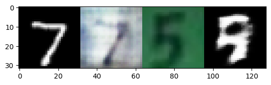
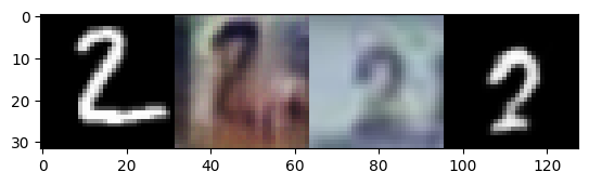
it[2100/4685] Loss_D:1.2505 Loss_G:6.9432 Loss_C:0.2115 elapsed_time:1.27mins it[2200/4685] Loss_D:1.9583 Loss_G:4.1971 Loss_C:0.2117 elapsed_time:1.33mins it[2300/4685] Loss_D:1.2686 Loss_G:6.8601 Loss_C:0.2186 elapsed_time:1.39mins it[2400/4685] Loss_D:0.8397 Loss_G:7.8509 Loss_C:0.2031 elapsed_time:1.45mins it[2500/4685] Loss_D:1.1641 Loss_G:8.0584 Loss_C:0.2072 elapsed_time:1.51mins it[2600/4685] Loss_D:1.1359 Loss_G:7.0753 Loss_C:0.2392 elapsed_time:1.56mins it[2700/4685] Loss_D:1.5548 Loss_G:6.8378 Loss_C:0.2235 elapsed_time:1.62mins it[2800/4685] Loss_D:1.0449 Loss_G:7.0575 Loss_C:0.2146 elapsed_time:1.68mins it[2900/4685] Loss_D:1.1044 Loss_G:8.0110 Loss_C:0.2093 elapsed_time:1.74mins it[3000/4685] Loss_D:0.8078 Loss_G:9.3036 Loss_C:0.2276 elapsed_time:1.79mins
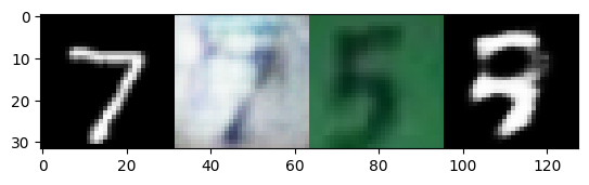
it[3100/4685] Loss_D:1.3796 Loss_G:8.1049 Loss_C:0.2373 elapsed_time:1.87mins it[3200/4685] Loss_D:0.9435 Loss_G:7.7675 Loss_C:0.2113 elapsed_time:1.93mins it[3300/4685] Loss_D:0.8737 Loss_G:8.0595 Loss_C:0.2316 elapsed_time:1.99mins it[3400/4685] Loss_D:1.1289 Loss_G:8.5881 Loss_C:0.2237 elapsed_time:2.04mins it[3500/4685] Loss_D:1.0201 Loss_G:8.1530 Loss_C:0.2123 elapsed_time:2.10mins it[3600/4685] Loss_D:0.9494 Loss_G:9.0783 Loss_C:0.2400 elapsed_time:2.16mins it[3700/4685] Loss_D:1.3046 Loss_G:8.9470 Loss_C:0.2160 elapsed_time:2.21mins it[3800/4685] Loss_D:1.2443 Loss_G:9.5515 Loss_C:0.2415 elapsed_time:2.27mins it[3900/4685] Loss_D:1.0502 Loss_G:8.8695 Loss_C:0.2037 elapsed_time:2.32mins it[4000/4685] Loss_D:1.2664 Loss_G:8.6817 Loss_C:0.2329 elapsed_time:2.38mins
it[4100/4685] Loss_D:0.9345 Loss_G:9.1384 Loss_C:0.1949 elapsed_time:2.46mins it[4200/4685] Loss_D:2.1560 Loss_G:3.3606 Loss_C:0.2013 elapsed_time:2.51mins it[4300/4685] Loss_D:1.1819 Loss_G:9.6243 Loss_C:0.2210 elapsed_time:2.57mins it[4400/4685] Loss_D:1.0053 Loss_G:9.8269 Loss_C:0.2121 elapsed_time:2.62mins it[4500/4685] Loss_D:0.9352 Loss_G:7.3601 Loss_C:0.2231 elapsed_time:2.68mins it[4600/4685] Loss_D:0.9737 Loss_G:8.8962 Loss_C:0.2206 elapsed_time:2.74mins
Discussion
The hardest part of this run was not the loss definition but getting the translated images to look convincing in both directions.
Quantitative evaluation
The implementation uses two generators and two discriminators, with the gray-to-RGB conversion handled explicitly through the helper functions. Because those helpers pass through NumPy, MNIST images had to move back to CPU before conversion. The discriminator padding was chosen so the output shape matched the BCE target tensors, and the cycle-consistency weight was kept at 10 as in the paper. During training, the cycle loss stayed fairly stable while the generator loss remained high, which already suggested that image quality would lag behind the cleaner parts of the loss curve.
Qualitative evaluation
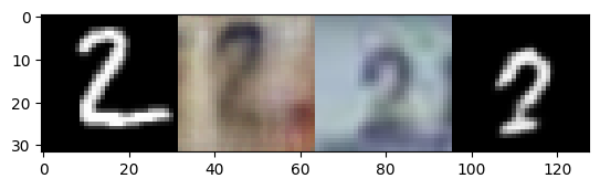
The translated images confirm that the harder direction here was MNIST to SVHN. The model preserved broad structure, but the RGB outputs still looked weak and blurry. Several factors could explain this behavior:
- increasing generator capacity, potentially with a U-Net style design
- using a cleaner or more consistent target dataset
- replacing the discriminator with a PatchGAN variant to reduce blurriness